💬Comments welcome. To leave a note, select any text and click the note / highlight button that pops up — or open the panel with the tab at the top-right (‹). Notes are visible only inside our private review group.
Course notes cut from Computational Photography, an AI-powered Slopendium for this lecture. Each section links back to its home in the book; sections marked optional go beyond what the lecture needs.
Contents · 31 sections on this page, from 15 chapters of the book
The pixel integral hands back a linear amount of light: double the aperture area or double the time and you double the number. Photographers almost never speak that way. They count light in stops, where one stop is a factor of two, because both the eye and the medium respond to ratios rather than differences (the same logarithmic story behind gamma encoding and Weber's law, Chapter 3.2, Perceptual color and trichromatic vision). A stop is the natural quantum of exposure: one doubling, one halving, one bit of light. Written on the log$_2$ scale the integral lives on, the whole messy business of exposure becomes simple addition and subtraction.
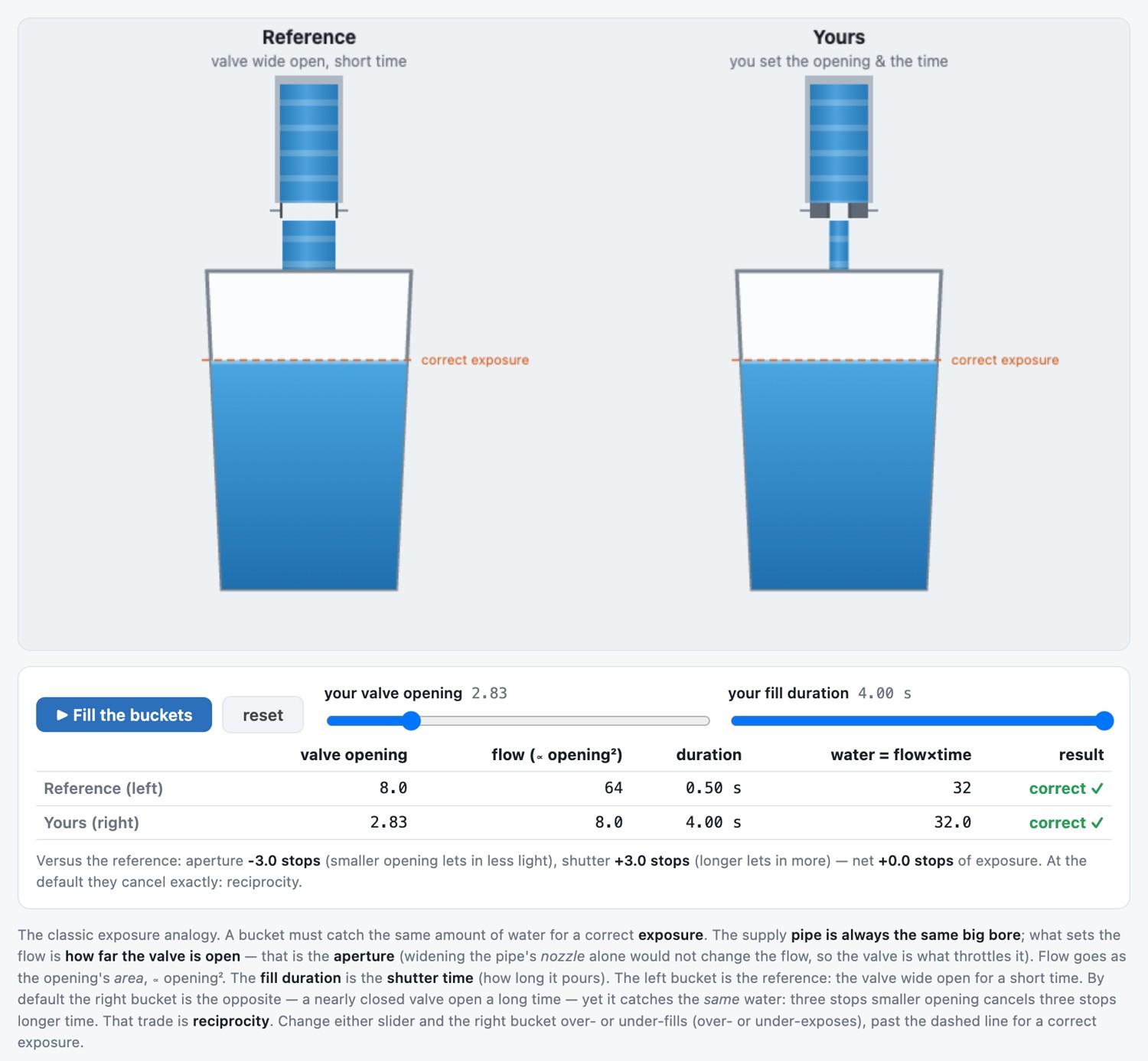
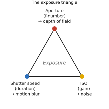
The power of the unit is that it is the same unit on every axis of the integral. One stop of aperture (a $\sqrt2$ step in the f-number, since light goes as $1/N^2$, Chapter 2.3, Lens image formation), one stop of shutter (a factor of two in time $t$), and one stop of ISO (a factor of two in gain) all change the brightness by the identical factor of two, so they can compensate one another in output brightness over an unclipped, approximately linear range. They do not preserve motion blur, depth of field, photon count or read-noise behavior. That commensurability is exactly what lets the three trade against one another, the exposure triangle: give back a stop of light on one leg, take it up on another, and the intended output brightness can remain unchanged. Many different aperture-shutter-ISO combinations therefore land on the same brightness, a redundancy photographers call equivalent exposures and rely on constantly (the faucet-and-bucket reciprocity of Chapter 5.2, Exposure and capture timing).
To name a whole family of equivalent settings with a single number, photography uses the exposure value (EV):
$$ \mathrm{EV} = \log_2\!\frac{N^2}{t}, $$
the base-2 logarithm of squared f-number divided by exposure duration expressed in seconds. EV describes aperture and shutter settings; relating it to scene luminance also requires ISO and meter calibration. One EV is one stop. Every $(N, t)$ pair on the same EV describes the same exposure, so a single EV names an entire diagonal of the aperture-shutter grid:
EV 13 (ISO 100)
$f/2.8$
$f/4$
$f/5.6$
$f/8$
$f/11$
$f/16$
shutter
1/1000
1/500
1/250
1/125
1/60
1/30
Read across: each stop you close the aperture is paid back by one stop of slower shutter, and the exposure never moves. Because EV folds the settings into one number, it doubles as a measure of scene light. At ISO 100 the same EV names how bright the scene is (sometimes called the light value): a meter's reading, $L = K N^2/(t S)$, is EV in disguise, and the old sunny 16 rule ("bright sun is $f/16$ at 1/ISO") is nothing but a printed EV chart, one EV per lighting condition.
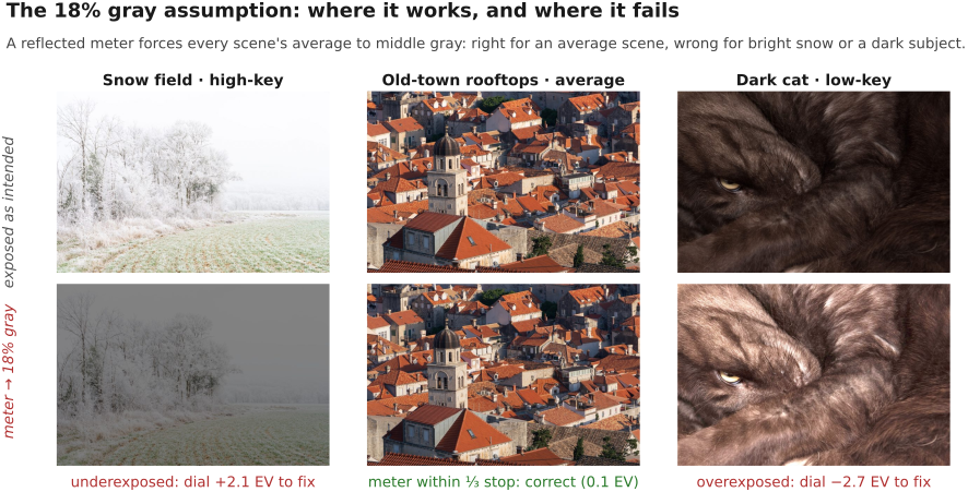
Once you have the unit, it turns up everywhere, which is the real reason to learn it. Meters report in EV, and every metered scene is placed on the EV ladder relative to mid-gray. Exposure compensation is dialed in EV ($+1$ EV to keep a snowfield white, $-1$ for a black cat), a direct nudge along the ladder. Auto-bracketing shoots frames at, say, $-2, 0, +2$ EV to merge into one high-dynamic-range image (HDR merging). A scene's dynamic range, a sensor's, a display's, are all quoted in stops (the ratio of brightest to darkest, in powers of two). Neutral-density filters are sold in stops (an ND8 is three stops), a lens's speed is "one stop faster," flash and studio lights meter in stops, and the noise story is a stop story too: because shot noise is set by photon count, every stop less light collected costs half the photons and a predictable step of signal-to-noise ratio (Chapter 2.8, Noise, signal-to-noise ratio and dynamic range). Stops and EV are the shared logarithmic language in which exposure, metering, dynamic range, filtration, and noise are all spoken; the full exposure and metering practice built on them is Chapter 5.2, Exposure and capture timing.
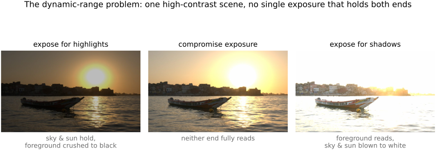
Two extremes bound what a single exposure can hold. At the top, a pixel's well saturates: once it has counted its full-well capacity of electrons, more light adds nothing and the highlight clips to white. At the bottom, the read-noise floor sets the dimmest signal still distinguishable from noise. The ratio of the two is the sensor's dynamic range: how much of a high-contrast scene a single exposure can capture. When a scene's range exceeds the sensor's (a bright window and a dim interior in one frame), no single exposure holds both ends, which is the motivation for high-dynamic-range (HDR) imaging, merging several exposures (Chapter 17.1, Dynamic range and multiple-exposure capture; Figure 2.8.14). Like everything else a photographer counts, dynamic range is quoted in stops (factors of two), which connects it straight to the exposure controls.
One subtlety keeps dynamic range from being the hard number it looks like: the bottom is not a sharp cliff where signal abruptly vanishes, but wherever the signal-to-noise ratio falls below what you are willing to accept. Engineers usually quote the engineering dynamic range, placing the floor at SNR = 1 (signal equal to noise); that is the most generous possible bound, and full-well divided by read noise approximates this criterion when read noise dominates at the threshold. With shot noise included, the electron signal $N$ at SNR $q$ solves $N/\sqrt{N+\sigma_r^2}=q$, giving $N_{\min}=(q^2+\sqrt{q^4+4q^2\sigma_r^2})/2$. The usable range is then $\log_2(N_{\mathrm{sat}}/N_{\min})$ stops, where $N_{\mathrm{sat}}$ is the effective saturation signal at the chosen gain. A photographer who wants genuinely clean shadows demands a far higher SNR, say 10 or 20, sets the floor higher, and counts fewer usable stops. This is why measurement sites report dynamic range at a stated quality threshold and their numbers disagree: the same sensor has a wide engineering range and a narrower photographic one. In this respect dynamic range behaves like depth of field: both carry a crisp-looking definition that actually rests on a chosen tolerance (an acceptable SNR here, an acceptable circle of confusion there), so the single figure you read off is only ever as hard as the criterion behind it.
There is one more limit that no sensor spec sheet lists: the lens. Bright parts of a scene scatter stray light inside the lens and camera body (faint reflections off every element surface, the diaphragm blades, and the barrel walls) that settle as a veil of light spread across the whole frame. This veiling glare, the diffuse cousin of lens flare, lifts the darkest tones off true black, adding a structured background and its shot noise. Even if the mean glare could be subtracted, its photon noise would remain; this differs from electronic read noise. It therefore caps the dynamic range a real photograph can reach below whatever the bare sensor could deliver, and it bites hardest exactly when dynamic range matters most, shooting a dim subject against a bright source. It is why lens coatings, hoods, and a clean front element buy real shadow contrast, and why the deepest blacks in a studio shot are easier to protect than those in a backlit scene. Flare and veiling glare get their full treatment as optical defects in Chapter 22.1, Aberrations and optical challenges (§10.1).
Figure 2.8.14(reproduced). The dynamic-range problem. One high-contrast scene (a sunset over water) developed at three exposures: expose for the highlights and the foreground is crushed to black; expose for the shadows and the sky blows out to white; the compromise loses both ends. No single exposure holds the full range: the motivation for high-dynamic-range merging of multiple exposures.
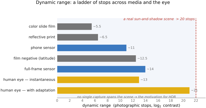
How wide a range, exactly? It helps to put numbers on it, because the dynamic ranges of real media and of the eye differ by a lot (Figure 2.8.15). A color slide is narrow, only about 5–6 stops; a reflective print about 6–7; a film negative is famously forgiving at roughly 12–13 stops of latitude; a phone sensor manages about 10–12 and a full-frame sensor about 14. The human eye sees about 10–14 stops instantaneously, but allow it to adapt (the slow re-centering of the retinal response covered with Chapter 3.3, Visual processing) and it spans 20+ stops over time; some animals do better still within their niche. Against all of these, an outdoor sun-and-shadow scene can exceed 20 stops in a single frame, which is precisely why no single capture holds it, and why HDR exists.
Figure 2.8.15(reproduced). *Dynamic range across media and eyes, as a ladder of stops: color slide (~5–6 stops), reflective print (~6–7), film negative (~12–13 latitude), phone sensor (~10–12), full-frame sensor (~14), and the human eye (~10–14 instantaneous, ~20+ once adaptation is allowed), with an animal example, set against a real sun-and-shadow scene exceeding 20 stops, which no single capture spans: the motivation for HDR.
Recovering an underexposed shot: full-frame vs. phone. The clearest demonstration is to underexpose one. Shoot the same underexposed scene as raw on a full-frame camera and on a phone, then push the exposure up in software by three or four stops (Figure 2.8.16). The full-frame frame cleans up (its deep full-well and low read-noise floor give it the headroom to be lifted) while the phone frame breaks into shadow noise and banding, because lifting the exposure also amplifies its read-noise floor, which sat much closer to the signal to begin with. At matched framing, exposure, and output resolution, this illustrates the benefit a larger total collecting area can provide; it is not a universal rule that sensor size alone determines dynamic range, and exactly why phones lean on burst capture and HDR+ (Multiple-exposure part) rather than trusting a single exposure. It is also a coding exercise: see Exercises & Experiments.
[figure fig-underexposure-recovery-ff-vs-phone not built]
Figure 2.8.16(reproduced). (Deferred, to be generated.) The same underexposed scene, shot as raw on a full-frame camera and on a phone, then pushed up about 3–4 stops in software: the full-frame frame cleans up (deep full-well, low read-noise floor → wide dynamic range), while the phone frame reveals amplified shadow noise and banding (its read-noise floor lifted with the signal): dynamic range scaling with sensor size.
💡 Big lesson (L2.46) — dynamic range = full-well capacity ÷ noise floor
A single exposure records from a top (the photosite's full-well capacity, where it saturates and clips to white) down to a bottom (the noise floor, the read noise that drowns the shadows). Their ratio is the dynamic range, quoted in stops. That floor is not absolute: it sits wherever the SNR drops below what you deem acceptable, so, just as with depth of field and its circle of confusion, the number depends on the quality criterion you pick (SNR = 1 gives the generous engineering range; a stricter SNR gives the narrower usable one). You widen it with a bigger well (larger photosites, why a full-frame sensor out-ranges a phone) or a lower floor (cooling, lower read noise), and you beat it altogether by merging multiple exposures (HDR). This is the capture-side companion to the quantization lesson below: what bounds a single shot is this range, full-well over floor, not the number of bits.
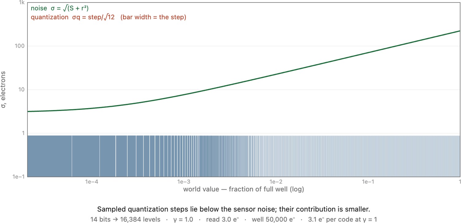
This is also the right moment to deflate a worry beginners often have about digital capture: that the image is quantized into a finite number of levels, and that this stair-stepping is what limits quality. With adequate raw bit depth and noise comparable to a code step, quantization is often a smaller limitation than sensor noise. Aggressive tonal edits or insufficient precision can still expose banding.
💡 Big lesson (L2.47) — quantization is rarely the real problem
With enough bits and a sane encoding, what limits image quality is noise and dynamic range (the two quantities of this section), not the number of levels the analog-to-digital converter (ADC) offers. The noise floor and the full well bound what you can record; the quantization step, once it sits below the noise, is invisible. (Indeed, a little noise dithers the quantization, hiding it further.) Levels matter in one place: banding in the deep shadows of a linearly-encoded image, too few codes where the eye, working in ratios, is most sensitive, and that is exactly the problem gamma encoding exists to solve, by spending code levels perceptually (Chapter 4.1, Color space 101). So "rarely" is not "never." We meet this lesson again in BASIC → Image representation → Float vs 8-bit, where floats with headroom are the sane default.
Figure 2.8.17(reproduced). The quantization step against the noise it has to beat (interactive). Both are standard deviations in the same units, so they can be compared directly: photon noise is Poisson, so $\sigma=\sqrt{S+r^2}$ electrons at a signal of $S$ electrons with read noise $r$, while one code step contributes $\sigma_q=\text{step}/\sqrt{12}$. The bars are the code steps and their width is the step itself, uniform under $\gamma=1$, squeezed into the shadows as $\gamma$ rises. Where a bar pokes above the noise curve, quantization is adding something the sensor was not already contributing; everywhere else it is buried, and the noise dithers it away. The scenario buttons set plausible hardware: a 14-bit linear raw from a good mirrorless, an 8-bit gamma-encoded JPEG from the same camera, and an 8-bit phone file whose pixel holds an order of magnitude fewer electrons. In the first three every step sits under the noise. Only 8-bit linear crosses, and only in the deepest shadows, the one place the lesson allows for, and exactly what gamma encoding exists to fix. Read noise, full well, bit depth and gamma are all adjustable, and the vertical axis can be read in electrons, as a fraction of the well, or in JNDs.
These three facts (that noise is the jitter of a photon count, that the signal-to-noise ratio is worst in the shadows, and that dynamic range is the full-well-over-floor a single exposure can hold) recur on nearly every later page: in how a photographer exposes to the right, in high-dynamic-range merging (Multiple-exposure part), and in the denoising of the basic pipeline. With measurement and its limits now in hand, the part turns next to what a second viewpoint buys you (depth), and then to the eye that will finally judge the result.
For an unchanged scene and lens transmission, optical exposure scales as
$$H\propto \frac{t}{N^2},\qquad N=\frac{f}{D}.$$
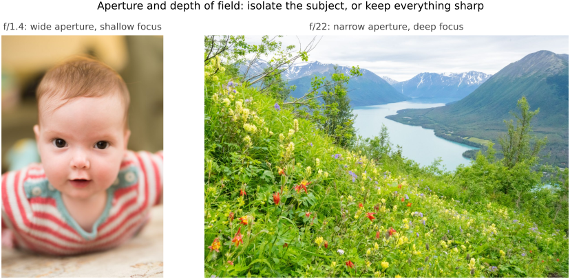
Twice the integration time collects twice the light. Multiplying the f-number by $\sqrt{2}$ halves it. Thus f/2.8 at 1/250 s and f/4 at 1/125 s give approximately the same optical exposure, but the longer integration blurs motion more and the smaller aperture increases depth of field.
A stop is the base-two logarithm of a light ratio. The setting-based exposure value uses time in seconds:
Increasing this EV by one halves optical exposure. Positive exposure compensation is a different convention: it asks an automatic mode for a brighter result relative to its metered choice. In aperture priority at fixed ISO, +1 stop will ordinarily double time. In manual mode with Auto ISO it may instead double gain while leaving the light collected unchanged.
ISO is not a third optical control. At fixed aperture and time, increasing gain scales the signal and its shot noise together. It can reduce the importance of noise added downstream of that gain, or select a sensor conversion-gain mode with lower input-referred read noise. It can also reduce highlight headroom. On an ISO-invariant sensor over the relevant range, low-ISO raw data brightened later can be close to a higher-ISO capture. The comparison in Chapter 2.8, Noise, signal-to-noise ratio and dynamic range applies only after matching output brightness and checking clipping.
The common association between high ISO and noise usually includes a reduction in collected light: we raise ISO because the scene is dim or the shutter must be fast. Add light, open the aperture or lengthen time when the photograph permits it. Raising ISO alone does not improve photon statistics.
Reflected-light metering measures light coming from the scene; it cannot separate a dark object in strong light from a pale object in weak light without additional information. Spot metering makes the chosen patch explicit. Evaluative metering uses more of the frame and may use recognized subjects. A gray card is a useful reference under the subject's illumination, not proof that a meter assumes exactly 18% reflectance. Snow and dark clothing are good tests of when compensation is needed.
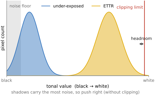
Expose to the right means collecting more light while retaining the highlights that matter. It is useful when time, aperture and saturation allow it; it is not a requirement to force every histogram against the edge. A longer exposure that blurs the subject is a poor trade for cleaner shadows. Inspect individual channels when possible, because a colored light can saturate one channel before the luminance preview looks white. Keep a margin when the camera's warnings refer to a processed preview rather than raw data.
💡 Big lesson (L5.1) — photographers measure light in stops
A stop is a factor of two. Time steps by two and f-number by $\sqrt{2}$. ISO and a software exposure slider can change rendered brightness by a stop without collecting another photon.
The f-number normalizes the physical opening by focal length. At the same f-number, a longer lens has a proportionally larger entrance pupil. For an extended scene of equal radiance, that compensates for the change in image scale so the on-axis irradiance is approximately unchanged, apart from transmission and close-focus effects. Aperture diameter alone would not give that useful comparison across focal lengths.
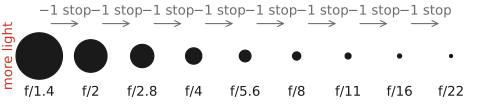
The familiar series f/1.4, f/2, f/2.8, f/4, f/5.6, f/8, f/11, f/16 follows from area. Each full-stop step multiplies the f-number by about the square root of two and therefore halves optical exposure at fixed time. Doubling time compensates for that step. For example, f/4 at 1/250 s and f/5.6 at 1/125 s collect approximately the same light per sensor area, with different motion blur and depth of field. Equal collected light does not make them interchangeable photographs.
A polarizer changes the mixture of polarized light reaching the sensor. Rotate it while watching reflections from water, glass or foliage. Its effect depends on the illumination and viewing geometry; it cannot remove every reflection. A photographic circular polarizer combines a linear polarizer with a quarter-wave plate to accommodate polarization-sensitive camera optics. It does not restore light hidden by a reflection; it selects a different measurement before that mixture is recorded.
A neutral-density (ND) filter reduces light so we can use an otherwise saturating time or aperture. If the filter removes $k$ stops, the same optical exposure requires
$$t_{\mathrm{ND}}=2^k t_0$$
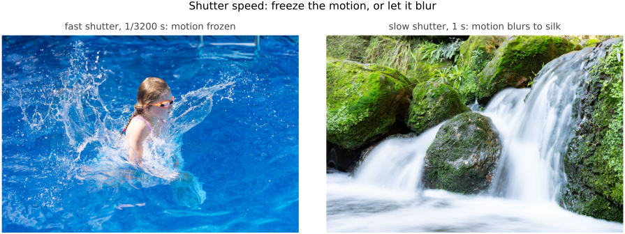
at unchanged aperture. A six-stop filter turns 1/64 s into 1 s. The water then blurs over one second while a static rock remains stationary. Darkening an unfiltered, clipped one-second exposure in software cannot reproduce the measurement. A variable ND uses polarization optics and can introduce uneven attenuation or color shifts.
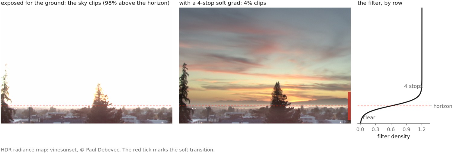
A graduated ND attenuates one region, often the sky, to fit a larger scene range into one exposure. It works best when its transition matches the scene; mountains and buildings crossing it can be darkened undesirably. Bracketing offers a different compromise when motion and alignment permit it. A protective filter adds a surface that may introduce reflections, so check it when photographing bright lights.
[figure fig-lens-filters not built]
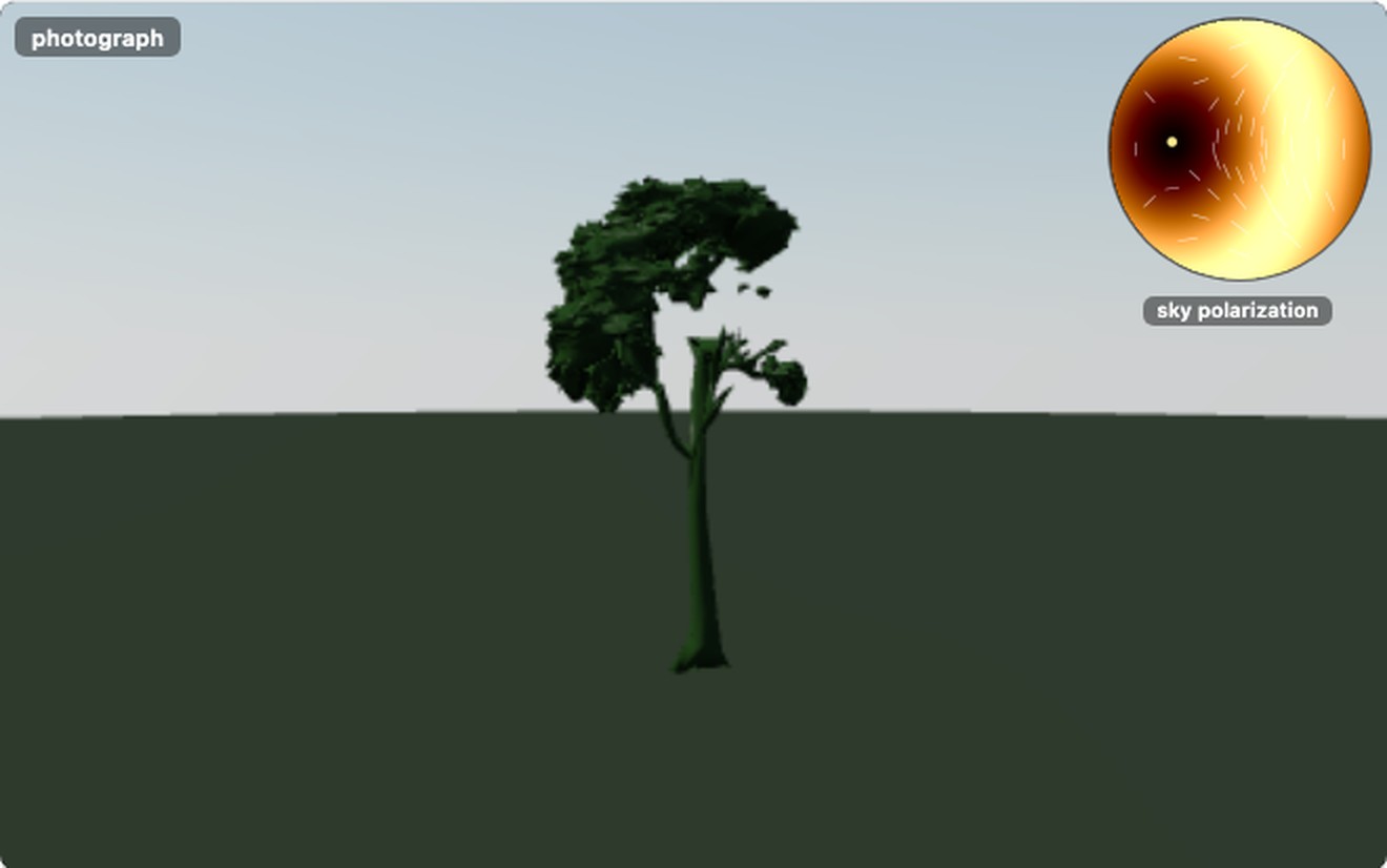
Figure 5.3.7(reproduced). The three image-altering filters. (Left) a circular polarizer rotated through its range: glare and reflections off water and glass vanish, the blue sky darkens, and saturation rises, strongest in the band ~$90°$ from the sun. (Middle) a strong ND turning a bright daytime scene into a long exposure (silky water) at a slow shutter. (Right) a graduated ND aligned to the horizon, holding back the bright sky so the whole high-contrast scene fits one exposure, with hard vs soft vs reverse edges. A polarizer's effect cannot be reproduced afterward, and a graduated ND's only where the sky was not already clipped.Figure 5.3.8(reproduced). Interactive. Why a polarizer makes foliage greener rather than merely darker. A leaf returns light two ways. Light that enters the waxy cuticle and scatters among the chlorophyll comes back green and depolarized, having bounced many times. Light that reflects off the cuticle without entering keeps the color of whatever lit it, outdoors a blue-white sky, and is polarized, because Fresnel reflection favors one component over the other. That second layer is a veil of sky-colored light lying on a saturated green, and the veil is what the filter takes off; the green underneath loses only the share of unpolarized light any polarizer absorbs, which is why, at matched brightness, the leaves gain saturation rather than merely losing brightness. Everything here is simulated rather than photographed: sun plus 34 sampled sky directions, each carrying the polarization Rayleigh scattering gives it, strongest about $90°$ from the sun, with the surface reflection evaluated through the Fresnel term that creates the polarization in the first place. The histogram measures saturation over the foliage pixels alone. Rotating the filter to crossed recovers about half the saturation the veil costs when the sun is low and the view crosses that band, and about a third at midday, because a polarizer removes only the polarized fraction and never the whole veil. Tree and grass models generated with Meshy AI. Interactive: set the filter angle or jump to the best one, move the sun by time of day, day of year and latitude, turn the scene, choose broadleaf, conifer, olive or a patch of grass, and switch the view between the photograph, the specular veil alone, and the sky's degree and angle of polarization.
Optional background: stabilization as an actuator
A stabilizer can deliberately move the image as well as counter shake. Bando and Holtzman Bando & Holtzman 2011 used this control to shape blur. Deliberate coded motion is a different capture strategy from trying to hold an image stationary.
Start with one source and decide where its shadow should fall. Add fill if that shadow is too dark for the intended picture. Add a rim or background light only if separation needs it. A good setup can contain one light; the names describe functions, not a minimum equipment list.
In a key-plus-fill setup, specify what a quoted lighting ratio compares. The ratio of lamp outputs is not the ratio of illumination on the two sides of a face: the bright side can receive both key and fill, and reflected light arrives from the room. Measure or inspect the subject under the combined illumination.
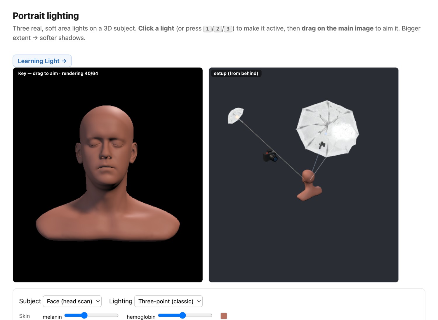
The portrait simulator lets us move the key and vary its extent while retaining the same face. Compare the shadow edge, eye sockets and specular highlights separately. “Butterfly,” “Rembrandt” and “split” are useful names for recurring shadow patterns, but a light placement should serve this person's face and the photograph's purpose.
Figure 5.4.5(reproduced). Try it yourself (web edition). A live portrait-lighting simulator: three soft area lights, a key, a fill, and a kicker, each with its own direction (azimuth, elevation), size, intensity, and color, sculpt a 3D face, with area-light-supersampled soft shadows and a physiologically grounded melanin/hemoglobin skin model. A second "from behind" view shows the lights as studio umbrellas plus the camera so you can read the whole setup, and one-click presets (butterfly, loop, Rembrandt, split, clamshell, rim) let you feel how a light's placement and size, not brightness, shape a face. In the printed edition this stands in as a screenshot. The 3D studio umbrella is generated with Meshy AI.
The lighting names identify jobs:
Light
Job
Key
Establishes the main direction and shadows
Fill
Supplies light to shadows left by the key
Rim, kicker, or hair light
Produces an edge or highlight that can separate subject and background
Background
Sets the backdrop independently of incidental spill
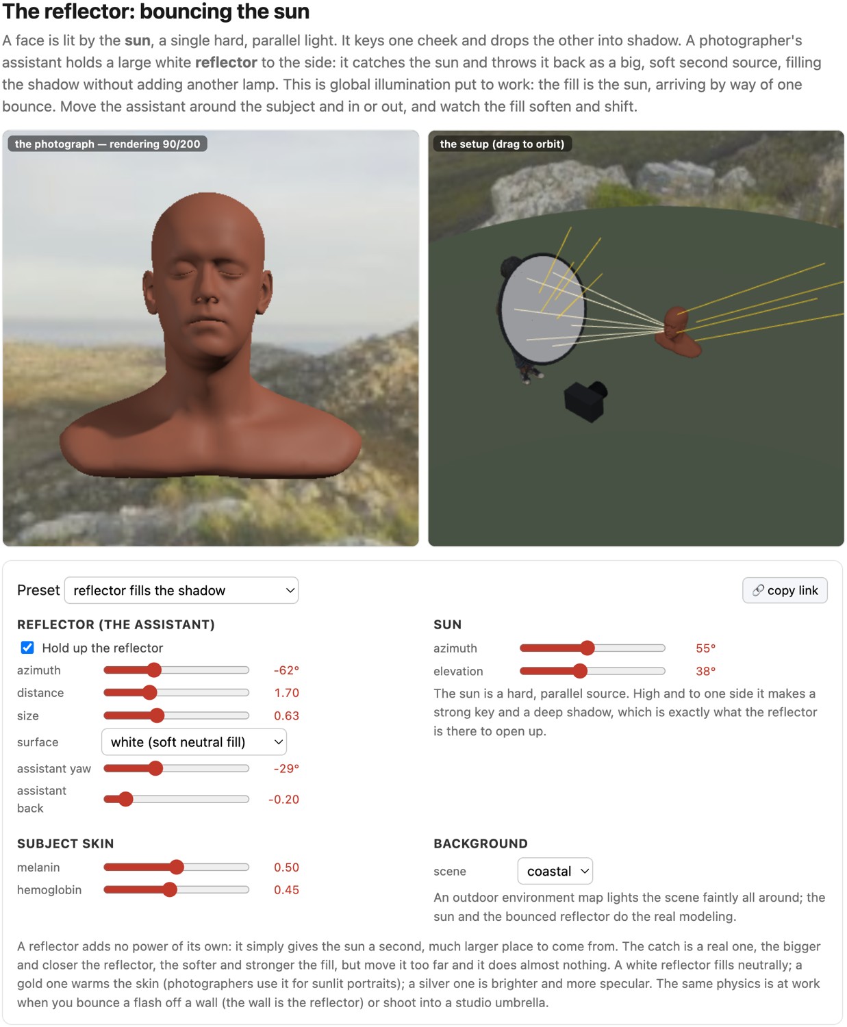
Three-point lighting combines key, fill, and rim. It is a common arrangement, not a minimum requirement. A reflector can do the fill's job without a second powered source. Separating the jobs makes adjustment easier: a brighter background need not require a brighter face.
Portrait-pattern names describe shadows on the face. Butterfly lighting places a small nose shadow below the nose; loop lighting moves that shadow sideways; Rembrandt lighting produces a lit triangle on the shadowed cheek; split lighting divides the face more strongly into lit and shadowed halves. Clamshell lighting combines a source above with fill below. The exact placement depends on the face, pose, and source size. Use the name to describe the observed pattern rather than treating a fixed angle as a recipe.
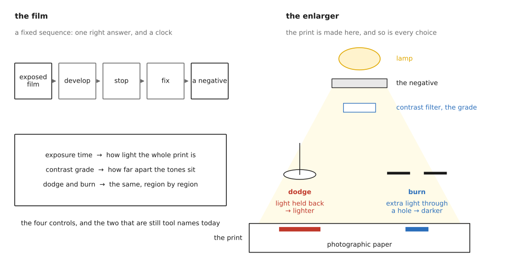
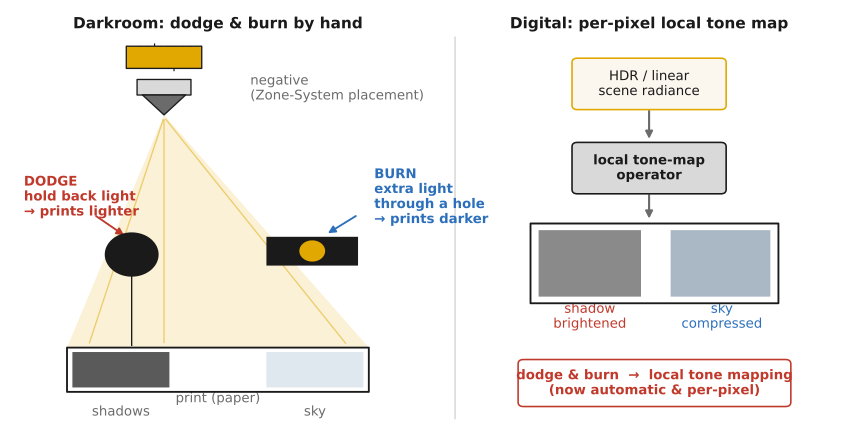
In the black-and-white negative process, development turns exposed silver-halide grains into metallic silver, and fixing removes remaining light-sensitive material. Printing exposes photographic paper through the negative to obtain a positive image. The print is a second exposure, with its own contrast and local adjustments.
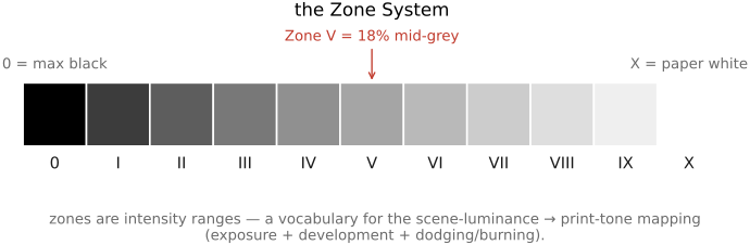
Dodging holds back enlarger light to make part of the print lighter. Burning adds light to make it darker. These operations give the familiar software tools their names. The Zone System connects decisions at capture and development to the tones wanted in the print Adams, The Negative. The historical connection is useful because it makes a practical point: a recorded negative does not specify one inevitable finished appearance.
Figure 5.5.1(reproduced). (Deferred: to be generated.) The chemical darkroom. (Left) the film pipeline: develop → stop → fix → a negative. (Right) the enlarger projects the negative onto photographic paper; the printer controls overall exposure time (lightness) and contrast grade (filter/paper), and shapes regions by dodging (holding light back → lighter) and burning (adding light → darker), the operations that name today's editing tools.
Under the enlarger, printing time controls how much exposure the paper receives. Paper grade, or filtration used with variable-contrast paper, changes the relation between negative density and print tone. A moving hand or paddle holds back light locally for dodging; an extra local exposure burns a region darker. A stop bath halts development before fixing removes the remaining light-sensitive material. These are distinct stages with distinct controls.
Two printers can start from the same negative and make different prints by changing those decisions. The negative is the recorded material; the print is its interpretation for a particular paper, light, and purpose. This is the practical meaning of comparing the negative to a score and the print to a performance. Digital development preserves that freedom while making many of the settings easier to record and repeat.
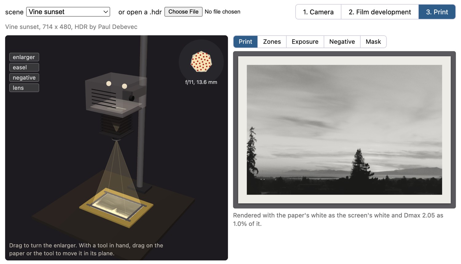
The whole chain can be tried in a simulator (Figure 5.5.2). It starts from a high-dynamic-range scene, so the camera records a real range of luminances, and follows Adams's three books in order: expose the negative, develop it, print it.
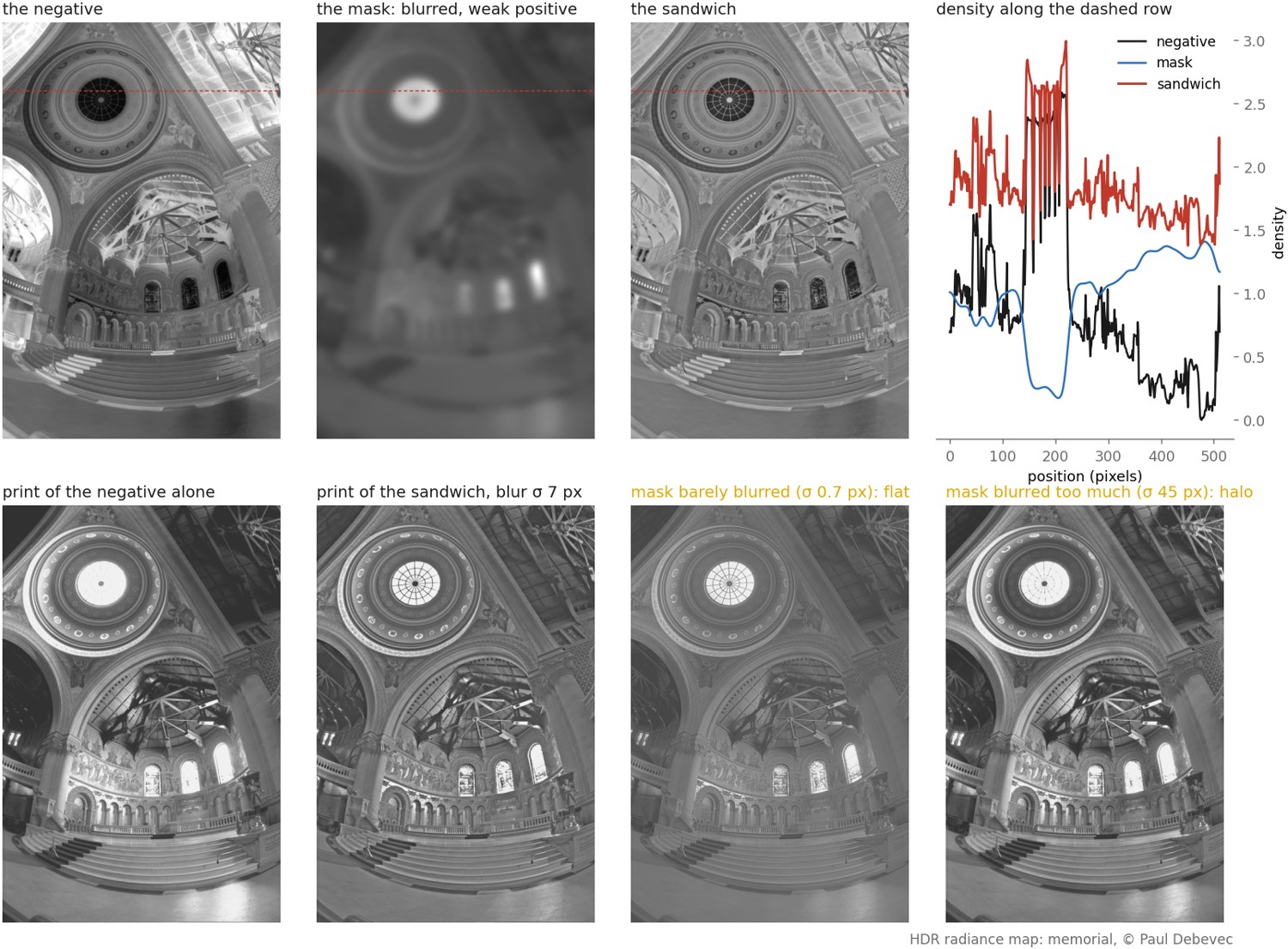
Figure 5.5.2(reproduced). A black-and-white darkroom, simulated from an HDR scene or your own .hdr file, in three tabs. Camera: choose a film, a color filter and a graduated ND filter, spot-meter a value and place it on a zone, and pre-expose if the shadows need it. Film development: developer, time, temperature and agitation set the negative's contrast from N−2 to N+2, shown on its characteristic curve. Print: a 3-D enlarger projects the negative through a lens of finite aperture onto graded or variable-contrast paper. Dodging and burning tools cast shadows with an umbra and a penumbra, each print pixel adds up the light it receives over the exposure, and an unsharp mask can be sandwiched with the negative. Notes after Adams suggest what to dodge and burn, and a tone-reproduction diagram chains the three transfer functions. The film, developer and paper responses are models.
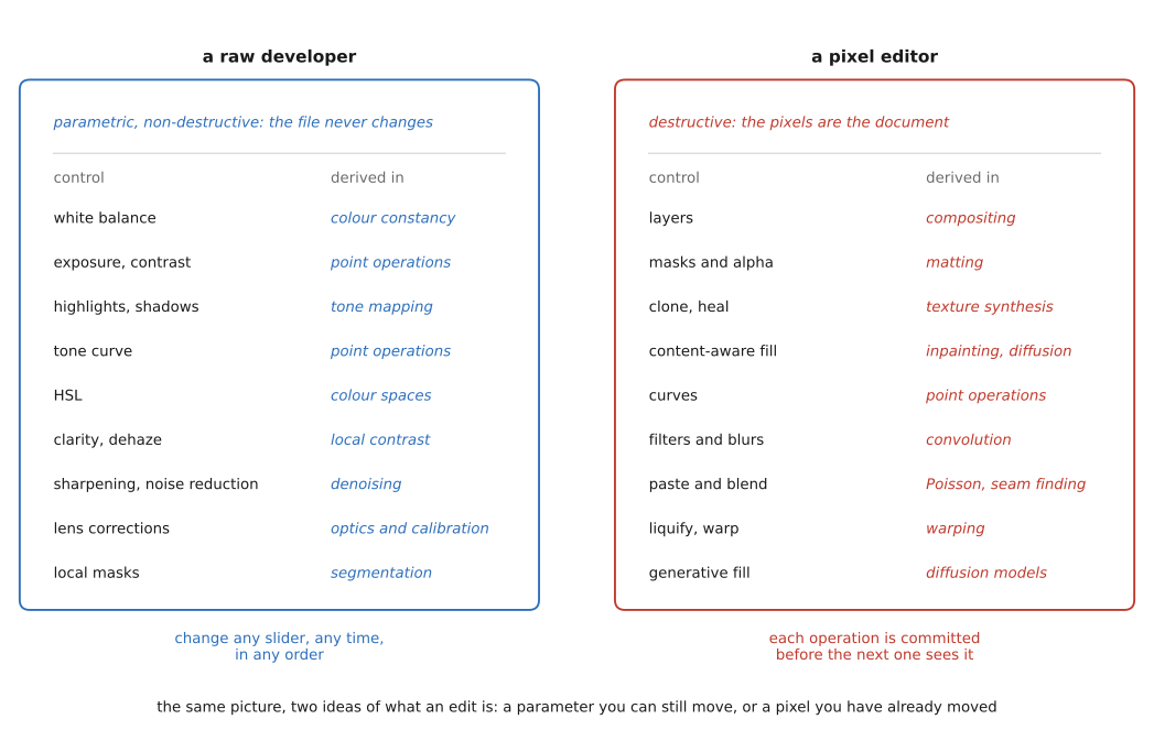
A parametric developer stores a recipe applied to source data. A layered editor stores image elements, masks and operations in a document. These approaches overlap: developers have local masks and retouching, and layered editors can retain reversible adjustment layers and embedded raw sources. The useful distinction is what can be revised and reproduced, not whether an edit is global or local.
Begin by selecting a frame whose expression, focus and motion are suitable. Check highlight clipping and the darkest important detail before spending time on polish. Set white balance for the intended rendering, correct geometry when needed, then establish overall lightness and contrast. Local adjustments can separate the subject or control a bright window without forcing the rest of the frame to follow the same curve. Revisit earlier choices when they interact.
Noise reduction and sharpening should support the intended output. Strong denoising can erase fine structure; sharpening can emphasize both texture and noise. A lens profile can correct systematic geometry or falloff, but resampling changes sampling density and brightening corners also amplifies their noise. “Correction” is still an operation with a cost.
Save a master with enough precision and a documented color interpretation. Export a separate version for the destination, including its color profile, dimensions and output sharpening. If masks depend on an external model or application cache, preserve those dependencies or save the rendered mask. The same recipe numbers can produce different pixels under another processing version.
Figure 5.5.3(reproduced). The two digital darkrooms, annotated with where each tool is explained in this book. (Left) a Lightroom-style develop panel: white balance, exposure/contrast, highlights/shadows, tone curve, HSL, clarity/dehaze, sharpening/noise reduction, lens corrections, local masks, labeled with the chapters that derive them (point operations, tone mapping, color constancy, denoising). (Right) a Photoshop-style workspace: layers, masks, clone/heal, content-aware fill, curves, labeled with theirs (convolution, Poisson/seam, diffusion). Parametric and non-destructive against pixel-level and compositing, though both can now make local, reversible edits: the difference is how the work is stored.
A parametric edit stores a recipe alongside the source rather than repeatedly replacing its pixels. For example, the recipe may record an exposure adjustment, a crop rectangle, and a local mask. Changing the crop later re-renders from the source instead of enlarging an already cropped export. Applying a common white-balance or rendering adjustment to a series likewise changes the recipes while preserving the captures.
This is different from claiming that every operation is reversible in an exported image. A JPEG export may clip highlights, quantize tones, and discard material outside the crop. The editable state survives because the source and recipe survive, not because the export contains enough information to undo every decision. Pixel layers, retouching strokes, and generated content may add further data that must also be retained.
A developer also helps manage a shoot: importing, comparing frames, rating, keywording, and applying a common recipe to a series. A layered editor is useful when the document must keep separate image elements, retouching, masks, or text. Many workflows use both. These are useful emphases, even though modern tools overlap and neither category is restricted to global or irreversible edits.
The control panel is a list of computational problems:
Photographic control
Computational connection
Exposure, levels, curves
Point operations and tone mapping
White balance and color mixer
Color transforms and illuminant estimation
Sharpening, texture, clarity
Filtering and local-contrast changes
Noise reduction
Statistical reconstruction
Raw development
Color-mosaic reconstruction and rendering
Crop, straighten, perspective
Coordinate transforms and resampling
Selections and local masks
Segmentation and spatially varying operations
Clone, heal, composite
Copying, reconstruction, and boundary matching
Generative fill
Conditional image synthesis
The names do not uniquely specify an implementation. A healing tool need not use the same algorithm as another application's healing tool. Learning the underlying problem lets us ask what information a control changes, which assumptions it makes, and which artifacts to inspect.
Two output constraints are easy to confuse. A print cannot emit the luminance of a sunlit scene, and its ratio between darkest and lightest regions may also be smaller. Scaling all values addresses the first mismatch but not the second. For a sense of scale, a sunlit scene with deep shade can span ten thousand to one or more, while a print under room light spans a few hundred to one at best. Tone mapping, local adjustments and lighting choices affect which distinctions survive.
A bright source can be suggested by a glow or surrounding dark tones even when the display cannot reproduce its luminance. That is a perceptual representation, not an absolute photometric measurement. Likewise, gamut mapping chooses a reproducible color when the target cannot display the original one. Chapter 18.10, HDR displays and display mapping and Chapter 4.7, Synthesizing color describe the output limits; Chapter 5.5, Developing and editing a photograph shows the photographer's choices within them.
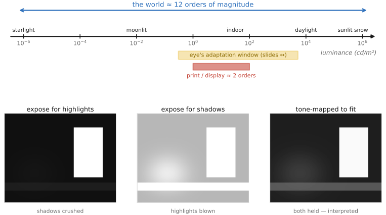
Figure 5.8.16(reproduced). The dynamic-range gap. A logarithmic luminance number line from 10⁻⁶ to 10⁶ cd/m² shows the real world's ~12-order span (starlight to sunlit snow); the eye's adaptation window slides along it (huge over time, far smaller at any instant); and the medium's ~2-order print/display band sits as a narrow stripe. Beside it, one high-dynamic-range scene rendered three ways, exposed for the highlights (shadows crushed), exposed for the shadows (highlights blown), and tone-mapped to fit, annotated with the historical compensations: Brunelleschi's silver sky and an added flare/glow standing in for a brightness no print can emit.
The history of depiction makes the intensity mismatch tangible. The lecture contrasts a painted sky with Brunelleschi's use of a reflecting silver surface for the sky in his perspective demonstration. A pigment and a reflection have different access to the surrounding illumination. Neither comparison can be reduced to an image's normalized pixel range.
The Zone System coordinates exposure, negative development and printing around planned tonal placements Adams, The Negative. Dodging and burning modify those placements locally. Characteristic curves compress the ends of the range, while perceptual tone-reproduction methods can also model visibility, glare or adaptation Ferwerda et al. 1996. These are distinct responses to limited output, not interchangeable names for a gamma curve. Retinex provides a related account of appearance through spatial relationships Land & McCann 1971, but it should not be read as proof that the eye simultaneously measures the entire luminance span across all environments.
Two prints from one negative can give different weight to a sky or a face. Dodging and burning change local emphasis, and a tone curve changes contrast relationships. The negative-to-print examples make that interpretation visible. For factual uses, keep track of whether the operation merely changes visibility or hides a relevant feature; the name of the tool does not settle the question.
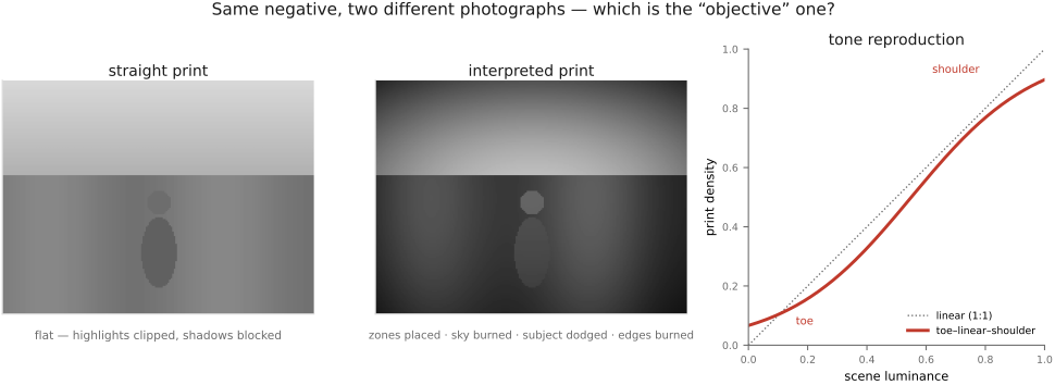
Figure 5.8.22(reproduced). The darkroom as authorship. One negative rendered two ways: a "straight" print (flat, the highlights clipped, the shadows blocked) and a fully interpreted print (zones placed, the sky burned down, the subject dodged up, the edges darkened), with a toe–linear–shoulder tone curve annotated alongside. Same latent image, two different photographs. Which is the "objective" one?
In a photographic print, dodging holds back exposure to make a region lighter; burning adds exposure to make it darker. The printer can use those controls to separate a face from its background, give a sky more weight, or reduce a distracting bright border. These are local decisions even when the negative is unchanged. Compare two prints of the same negative by following where the eye goes first and which details become legible, rather than asking only whether the global brightness matches. The operation changes the interpretation through visibility and emphasis (Figure 5.8.22). The printers of the twentieth century treated this as the work itself: W. Eugene Smith reportedly spent days printing a single photograph of Albert Schweitzer, and Ansel Adams burned the sky of Clearing Winter Storm heavily to give it weight. The same negative yields as many prints as there are printers and intentions.
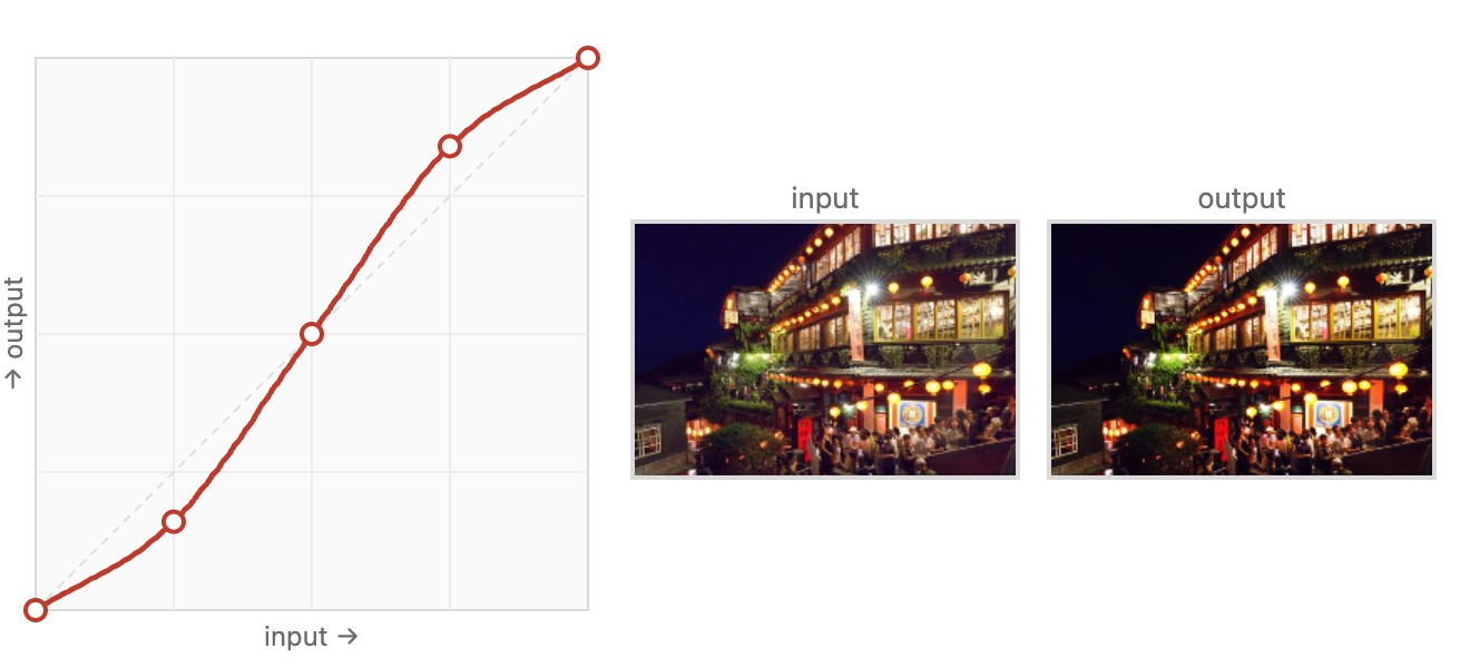
Exposure, contrast, and levels are all constrained shapes: a fan, a straight steepen, a clipped stretch. The most general point operation simply lets you draw the curve freehand: the tone curve tool gives you a handful of control points to drag wherever you please, and the editor threads a smooth interpolating curve through them (Figure 8.3.8). A monotone curve, one that never decreases, preserves the ordering of tones. A non-monotone curve deliberately reverses that ordering over part of its range, as in solarization effects. Catmull–Rom interpolation (Catmull & Rom 1974 (interpolating splines)) can overshoot even when the control points are ordered. Use a monotonicity-preserving interpolant when tone reversals must be excluded.
Figure 8.3.8(reproduced). The general tone curve. A few draggable control points (dots) are interpolated by a smooth monotone spline (solid) into an arbitrary transfer curve; the 45° identity is shown dashed. Because the spline is kept monotone (never decreasing), a brighter input never maps to a darker output, so tones cannot invert. This single freehand curve subsumes the exposure bow, the contrast steepen, and the levels stretch of the earlier figures.
Sidebar 1: splines (the math)
A spline fits a smooth curve through a set of control points (knots) $(x_i, y_i)$ by stitching together low-degree polynomial pieces: for our purposes one cubic per interval $[x_i, x_{i+1}]$, with the pieces joined for continuity. The cleanest way to write each piece is the cubic Hermite form. On $[x_i, x_{i+1}]$, set $t = \frac{x - x_i}{x_{i+1} - x_i} \in [0, 1]$ and write
The piece passes through $y_i$ at $t=0$ and $y_{i+1}$ at $t=1$ no matter what; the only free choice is the tangent (slope) $m_i$ at each knot, and that choice is what separates the schemes:
Catmull–Rom (interpolating, $C^1$): take the tangent as the centered difference $m_i = \frac{y_{i+1} - y_{i-1}}{x_{i+1} - x_{i-1}}$, local and cheap, but it can overshoot between knots and so go non-monotone.
natural cubic ($C^2$): demand continuous second derivatives and minimize the total curvature $\int (p'')^2$; this couples all the knots into one tridiagonal linear system for the slopes, the smoothest fit, but it too can overshoot.
monotone cubic (Fritsch–Carlson, Fritsch & Carlson 1980 (monotone cubic)): start from Hermite tangents, then clamp them so every segment is monotone. Write the secant slope $\Delta_i = \frac{y_{i+1} - y_i}{x_{i+1} - x_i}$; where a secant is flat ($\Delta_i = 0$) set the neighboring tangents to $0$, and otherwise keep $(\alpha, \beta) = (m_i/\Delta_i,\ m_{i+1}/\Delta_i)$ nonnegative and inside the circle $\alpha^2 + \beta^2 \le 9$. This guarantees no inversion, exactly the property a tone curve needs (brighter in $\Rightarrow$ brighter out), which is why it is the standard choice here.
B-splines are the approximating cousin: the curve follows a control polygon and need not pass through the knots, smoother and easy to keep monotone, at the cost of exact interpolation.
Sidebar 2: spline families (drag to compare)
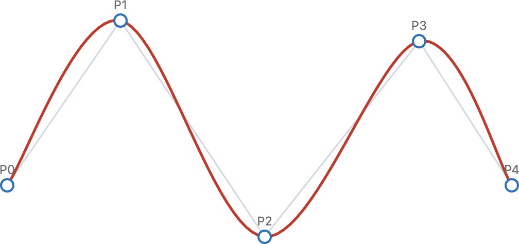
Figure 8.3.9.Spline families through the same control points. Piecewise-linear, natural cubic, and Catmull-Rom all interpolate (pass through every point); a B-spline only approximates, staying inside the convex hull of its control points. The Bézier option draws the same Catmull-Rom curve, written as cubic Bézier segments; the natural cubic and the B-spline are both $C^2$, the others only $C^1$ or $C^0$. The trade-off (interpolation vs smoothness, global vs local control) is the same one faced by the tone curve above and by the resampling kernels of a later chapter. Drag a point to feel how local each scheme is.
Sidebar 3: how analog photography shaped the same mapping
Long before a draggable digital curve, photographers controlled the scene-tone → printed-tone mapping entirely by physical and chemical means, and the modern tone curve is the digital descendant of that whole toolkit.
Exposure decides where a scene luminance is placed on the film's response: the Zone System's "place this shadow on Zone III and let the highlights fall where they may."
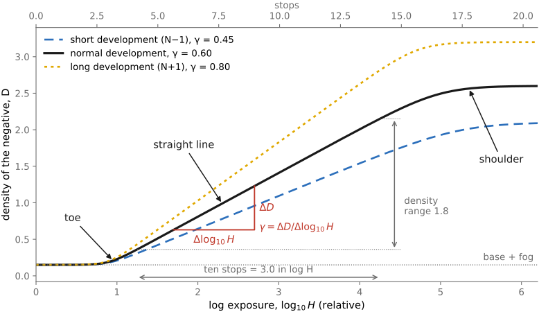
The film's characteristic (H&D) curve and its gamma / contrast are set partly by the emulsion and partly by development: time, temperature, agitation, choice of developer. Photographers deliberately push or pull (over- or under-develop) and use "N / N+1 / N−1" development to expand or compress the scene's tonal range onto the film.
Pre-exposure / flashing (a uniform sub-threshold exposure) lifts deep shadows above the film's toe, raising the floor without touching the highlights (the analog of a black-point lift).
At print time the paper grade (contrast grade 0–5) sets the print's slope, and local dodging and burning (holding back or adding light region by region) place each tone, the ancestor of the masked local point operations below.
The free-form tone curve, plus those masked local edits, is the digital reincarnation of this entire workflow. For the canonical treatment, see Ansel Adams' trilogy, The Camera, The Negative, and The Print, with the Zone System developed in The Negative.
A freehand tone curve subsumes everything earlier in the chapter (you could draw the exposure scale, the contrast steepen, or the levels stretch by hand) which is why it is the photographer's most general tonal tool. The tone-mapping chapter pushes the idea to its physical conclusion with principled, automatically chosen curves (the Reinhard operator $L/(1+L)$ and relatives, Reinhard et al. 2002) for compressing high-dynamic-range scenes; here we simply note that the general curve is the container they all fit into.
In some scenes the range of luminance is too high to be captured, let alone displayed, in a single picture: a sunlit window and the dim room around it, a street at night with its lamps, a landscape with the sun in the frame. The brightest parts that matter can be thousands of times brighter than the darkest ones, while a sensor records perhaps twelve to fourteen stops between clipping and noise, and a screen or a print shows fewer still. Expose for the highlights and the shadows sink into noise; expose for the shadows and the highlights clip to white. This part is about capturing such scenes anyway, by recording more than one exposure, or more than one kind of measurement, and combining them; the next part, Part 18, Tone mapping and display, is about showing the result.
The dynamic range of a sensor is the ratio between the largest signal it records before clipping and the smallest it can tell apart from noise, usually counted in stops (log base 2); Chapter 2.8, Noise, signal-to-noise ratio and dynamic range defines it and shows how noise and ISO set it. A display's range is defined the same way, between its brightest white and its darkest distinguishable black. High dynamic range has no quantitative definition. A scene, an image or a display is called HDR when its range exceeds what a standard sensor can record in one exposure or a standard display can show, so the threshold moves as the technology improves.
Modern sensors can deliver excellent dynamic range, especially with large sensors at low ISO, and single-capture HDR is often a reality. However, in many scenarios, a single snapshot is not sufficient.
HDR is one of the paradigmatic examples of a central idea of computational photography: when the technology cannot record what we want in one picture, capture several pictures that each record part of it, and combine them computationally. The same idea extends depth of field by merging photographs focused at different distances (Chapter 23.3, Focal stacks and depth of field extension), extends the field of view by stitching photographs aimed in different directions (Part 20, Field of view extension and panorama stitching), and reduces noise by averaging several frames of the same scene (Chapter 13.2, Denoising by averaging), or recovers resolution from their sub-pixel shifts (Chapter 14.2, Multi-frame super-resolution). HDR is also one of the first techniques to which the name computational photography was attached: Steve Mann, who coined the term in the mid-1990s, used it for work that included combining differently exposed pictures to extend dynamic range Mann & Picard 1995.
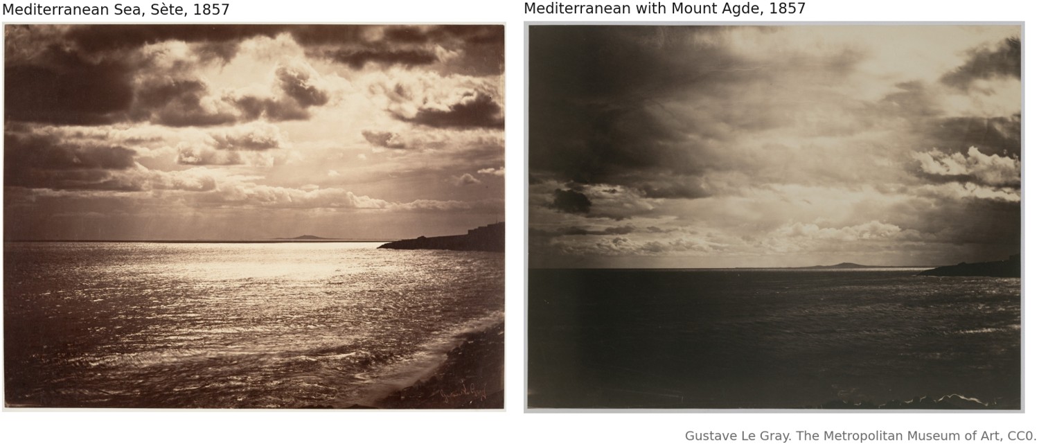
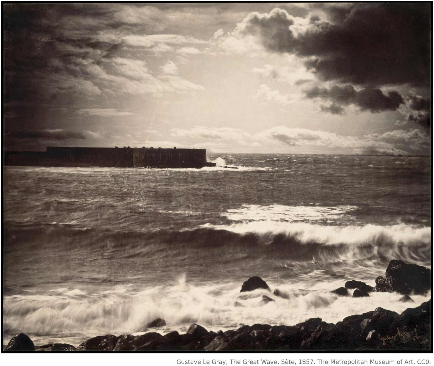
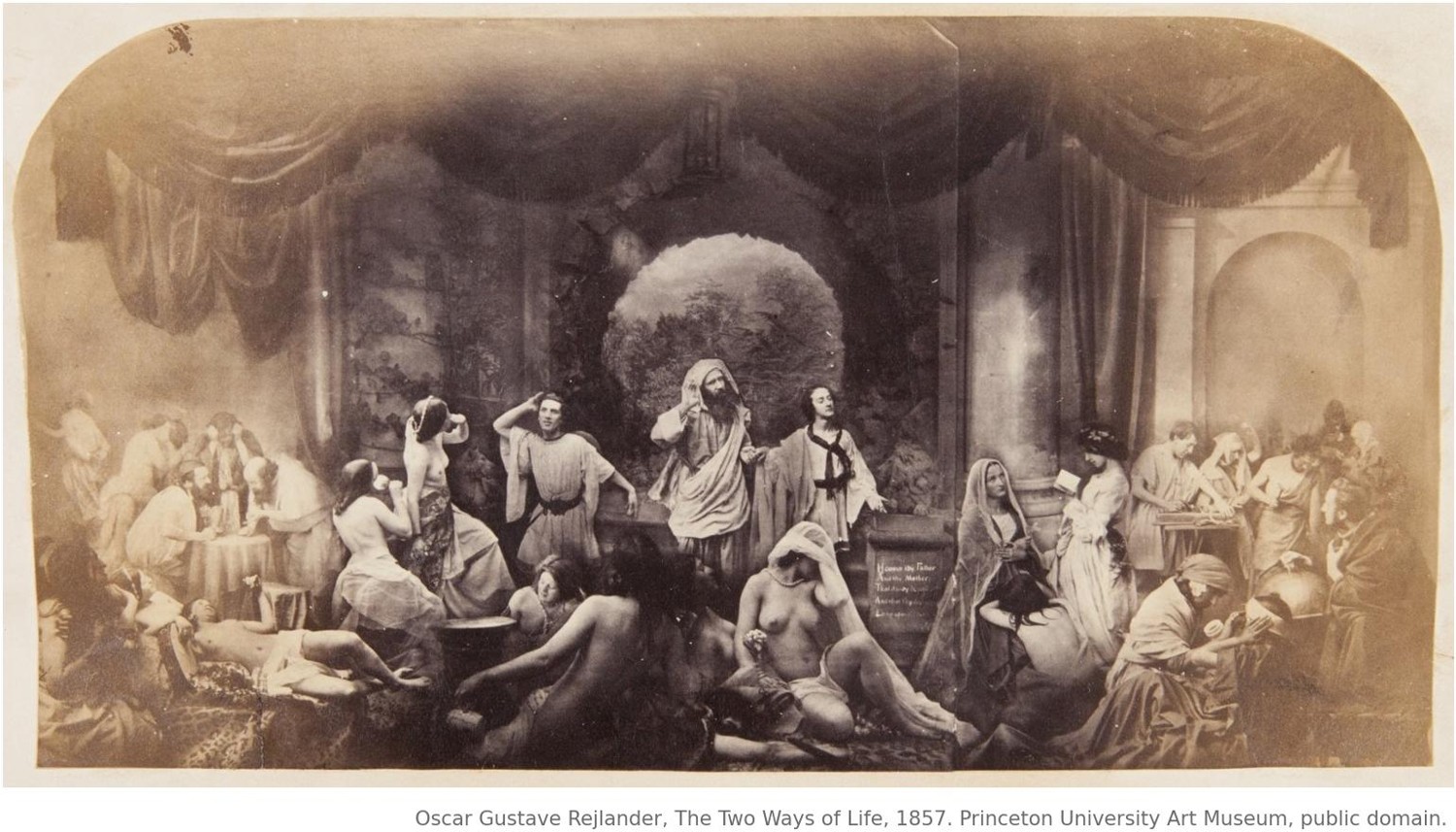
The idea of combining multiple exposures for dynamic range expansion is almost as old as photography. In the 1850s, Gustave Le Gray combined separate negatives for sea and sky to make seascapes that photographic materials struggled to record in one exposure. The Getty's examples even show the same sky negative used with different foregrounds (Getty exhibition). Combination printing was therefore both a response to capture limitations and a compositional choice. Modern HDR merging shares the idea of combining complementary exposures, while adding the requirement that registered measurements describe a common scene. Chapter 18.9, High dynamic range in traditional photography follows that craft further: lighting to reduce the scene's range, graduated filters, the Zone System, and dodging and burning under the enlarger.
Figure 17.0.1 shows two of his prints taken from the same spot at Sète, each printed from two glass negatives, under two different skies.
Figure 17.0.1(reproduced). Gustave Le Gray, Mediterranean Sea, Sète (left) and Mediterranean with Mount Agde (right), both 1857, albumen prints. Both show the same view, with Mount Agde on the horizon and the jetty on the right, and the museum catalogs each as printed from two glass negatives, one for the sea and one for the sky. The skies are clearly different. The seas differ too, sunlit in one and dark in the other, so this pair does not by itself show a negative reused; the Victoria and Albert Museum reports that prints of this view in other collections share one sea negative under several different skies. (The Metropolitan Museum of Art, CC0.)
HDR capture estimates a wider range of scene intensities than one exposure can usefully record; tone mapping renders that range for a particular display or print. Calibration and merging should preserve measurement relationships, while rendering chooses brightness and contrast for the viewer, which is why they are two parts. This one ends with a radiance map and the knowledge of where it is trustworthy. Part 18, Tone mapping and display takes it from there, along with the display encodings and gain maps that determine how the result survives distribution.
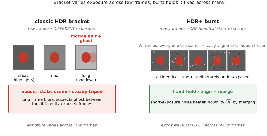
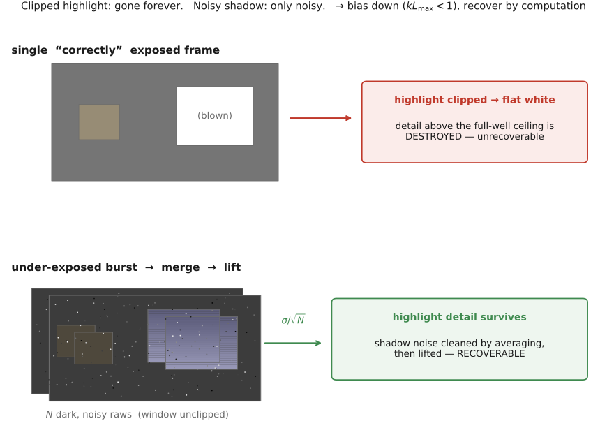
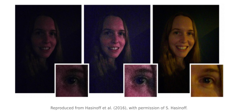
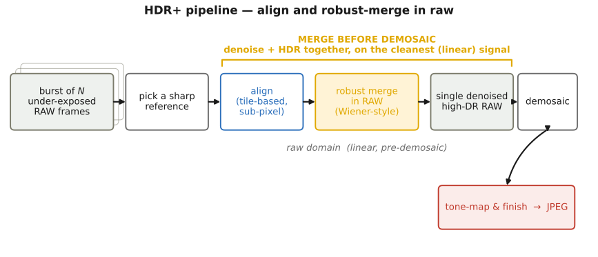
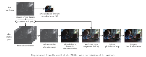
The chapters follow the capture pipeline. Chapter 17.1, Dynamic range and multiple-exposure capture sets out the gap between the scene, the sensor and the display, then how to capture a bracket: which exposure parameter to vary, what each choice costs, and how some sensors combine exposures on the chip. Chapter 17.2, Camera response and radiance calibration recovers the camera's response so that differently exposed frames can be compared in linear units, a step raw files make nearly free. Chapter 17.3, Merging exposures combines the calibrated frames into one radiance estimate, weighting each frame by how well it measures each pixel, and Chapter 17.4, Ghosts and motion deals with whatever moved between frames. Chapter 17.5, Single-shot range and inverse tone mapping covers sensors that deliver extra range in one frame and methods that estimate the missing range from a single image. Chapter 17.6, HDR+ and burst imaging on phones protects the highlights with a burst of short, identical exposures and averages them to recover the shadows. Chapter 17.7, Encoding HDR images closes the part with the file formats that store a radiance map and deliver an HDR photograph. Rendering the result, including exposure fusion, which skips the radiance map, and the darkroom craft that met the same problem before digital sensors, is the subject of Part 18, Tone mapping and display.
PS4 merges an exposure bracket into a radiance map and tone-maps it. → Chapter 1.5, Problem sets (appendix).
Dynamic range is the ratio between the largest and smallest signal a sensor records. At the bright end, charge capacity or the readout chain limits the recorded signal. At the dark end, noise sets a gradual loss of precision rather than a hard black threshold. The usable dynamic range depends on the minimum signal-to-noise ratio (SNR) accepted for the task (Chapter 2.8, Noise, signal-to-noise ratio and dynamic range). That chapter develops both ends: full-well capacity at the top (the maximum number of electrons a pixel can hold), read noise and photon noise at the bottom. The engineering definition places the floor where the signal equals the noise (0 dB), but that is too low for photographic purposes, where 30 dB is considered close to perfect and even 15 dB is severely noisy. Figure 17.1.1 shows examples. Like depth of field, quantitative dynamic range is a question of tolerance, to noise in this case. Recall that bright scene values that saturate the photoreceptor may still be read below the maximum because of electronic noise. The ability to capture high dynamic range can further be limited by the veiling glare inside the lens, which lifts the darkest tones before the sensor sees them.
Figure 17.1.1(reproduced). What a signal-to-noise ratio looks like: a 1:1 crop of a photograph, one image pixel per screen pixel, with noise at 0, 10, 15, 20, 30 and 40 dB, where the SNR in decibels is $20 \log_{10}$ of the signal over the noise, so 20 dB is a noise of one tenth of the signal. The noise is added in linear light and grows with the square root of the signal, like photon noise, and the stated SNR is that of an 18% gray: the bright seed head is cleaner than the figure says and the dark background noisier. At 0 dB, the engineering floor of dynamic range, the picture is barely usable; at 15 dB it is severely noisy; at 30 dB the noise is hard to see.
When the dynamic range of a scene exceeds that of the sensor, we capture multiple exposures to span the range. We may need to register these images in space (similar to denoising). Chapter 13.2, Denoising by averaging aligns and averages a burst of equal exposures, Part 12, Matching pixels across space and time covers the registration itself, and Chapter 17.4, Ghosts and motion deals with what moves between the frames of a bracket. We also need to calibrate the pixel values photometrically to bring them into the same absolute linear range proportional to scene-radiance values $L(x,y)$, which may require the calibration of the film or digital camera response curve (the beauty curve in particular, Why scene-linear looks dull in Part 8, Basic image processing and ISP; Chapter 17.2, Camera response and radiance calibration recovers it). Motion, clipping in every frame, or inadequate shadow exposure can leave parts of that estimate uncertain.
💡 Big lesson (L2.46)
A common sensor dynamic-range measure divides the saturation signal by the read-noise standard deviation, in consistent units. A stricter quality threshold gives a smaller usable range. Bracketing extends coverage when its exposures provide reliable, registered measurements of the same scene.
The gap between the scene, the sensor and the screen⧉
Distinguish the range within one scene from the much larger range encountered across daylight, interiors and night. Likewise, visual adaptation across time is different from simultaneous contrast sensitivity. A sensor's capture range and a display's visible contrast also depend on noise criteria, viewing conditions and hardware; one fixed ratio does not describe all of them.
With that caveat, some orders of magnitude help. A view from a dim interior through a window onto a sunlit street can span around 100,000:1, about 17 stops, between the brightest diffuse surface and the darkest shadow that still shows detail, before counting the sun or specular highlights.
Following the light from its source shows where such a number comes from. The disk of the sun has a luminance of about $1.6 \times 10^{9}$ cd/m², far beyond anything else in a photograph. A clear blue sky is around 5,000 to 10,000 cd/m², some two hundred thousand times dimmer. A white wall in direct sun receives about 100,000 lux and, reflecting most of it, has a luminance around 25,000 cd/m². In the shade, a surface sees the whole sky but not the sun: a uniform sky of luminance $L$ over a full hemisphere delivers an illuminance of $\pi L$, about 15,000 lux, so a mid-gray surface there is around 2,500 cd/m², ten times dimmer than the sunlit wall. Indoors, a surface near a window sees only the part of the sky the window frames. A one-square-meter window three meters away subtends about 0.1 steradian, so the illuminance drops to a few hundred lux, some forty times less than in the open shade, and a mid-gray surface is around 60 cd/m². Many points in the room do not see the window at all and are lit only by light bounced off the walls and ceiling, a few lux to a few tens of lux; a dark fabric there, reflecting five percent, is around 0.2 cd/m². From the sunlit wall outside to that fabric is about 25,000 / 0.2, or 125,000:1: the 100,000:1 above, reached by a chain of ordinary factors, each of ten or forty, and without the sun or the sky ever appearing in the frame.
No single exposure of such a scene holds both ends: Figure 2.8.14 develops one scene at three exposures.
Figure 2.8.14(reproduced). The dynamic-range problem. One high-contrast scene (a sunset over water) developed at three exposures: expose for the highlights and the foreground is crushed to black; expose for the shadows and the sky blows out to white; the compromise loses both ends. No single exposure holds the full range: the motivation for high-dynamic-range merging of multiple exposures.
The eye covers a far wider range, but not at once (Chapter 3.3, Adaptation and constancy). Across its states of adaptation, vision works from about a millionth of a candela per square meter, the threshold of fully dark-adapted vision, to sunlit snow at $10^{4}$ to $10^{5}$ cd/m², some ten or eleven orders of magnitude, well over thirty stops. At any one operating point it distinguishes far less, roughly four orders of magnitude, and it sees a high-contrast scene well because it moves: each fixation adapts to the part of the scene it lands on. A camera has to record the whole scene in one exposure, which is why 100,000:1 is a problem for it and not for the eye.
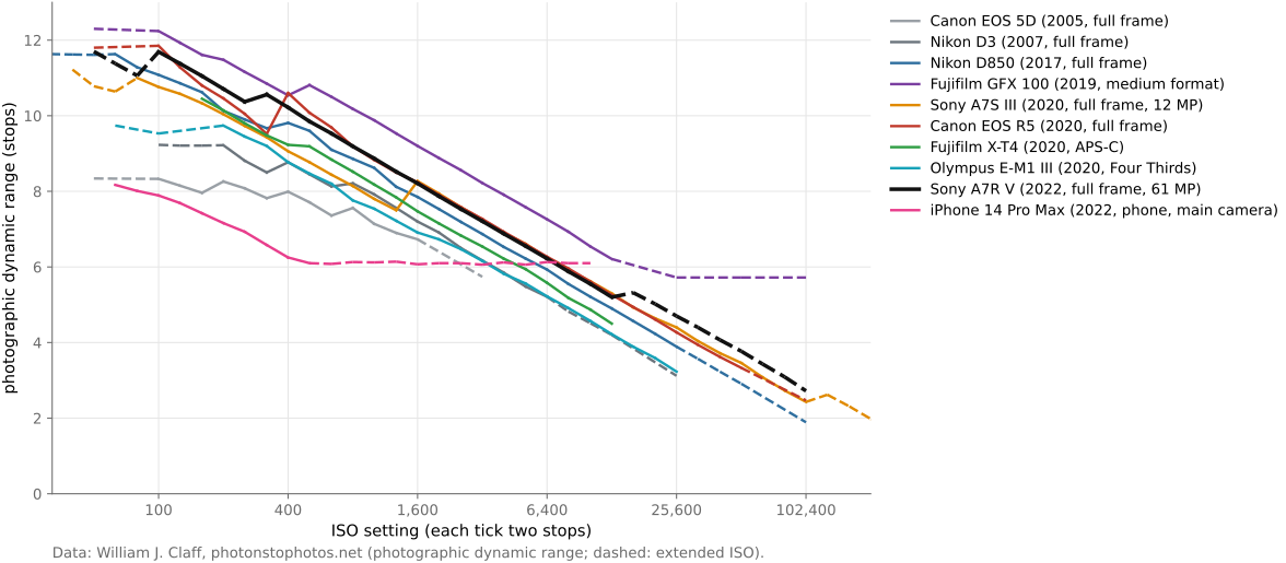
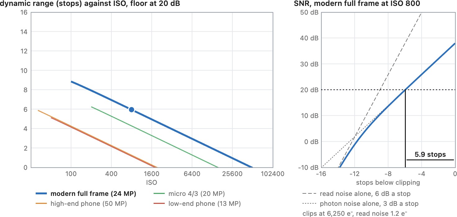
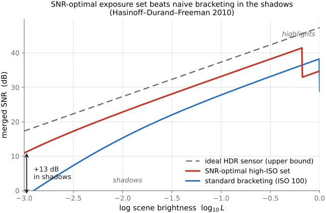
A current large-sensor camera at base ISO (the lowest ISO, i.e. the lowest gain) records roughly 12 to 14 stops between clipping and a noise floor at a signal-to-noise ratio of one, and a phone sensor fewer. That is the engineering definition, with the floor at 0 dB, where the signal equals the noise, which nobody would call a usable shadow. Raising the floor costs range quickly. With photon noise and read noise, the dimmest signal reaching an SNR of $q$ is $N_{\min}=(q^2+\sqrt{q^4+4q^2\sigma_r^2})/2$ electrons (Chapter 2.8, Noise, signal-to-noise ratio and dynamic range). For a full-frame pixel with a full well of 50,000 electrons and 3 electrons of read noise, the range is 13.8 stops at 0 dB, 11.6 stops at 10 dB (an SNR of about 3) and 8.9 stops at 20 dB (an SNR of 10). For a phone pixel with 6,000 electrons and 1.5 electrons of read noise, the same three floors give 11.5, 9.0 and 5.9 stops. At 20 dB the floor is set almost entirely by photon noise, about 100 electrons whatever the read noise, so the range is little more than the full well divided by 100, and what buys clean shadows is a deeper well, which means a larger pixel. Figure 17.1.2 shows how it falls with ISO for ten cameras.
Figure 17.1.2(reproduced). Dynamic range against ISO for ten cameras, from a 2005 full-frame DSLR to a 2022 phone, measured by William Claff as photographic dynamic range: from clipping down to the level where noise becomes objectionable in the whole image seen at a fixed size, rather than to a signal-to-noise ratio of one. That lower floor is why the values sit below the 12 to 14 stops of the engineering definition, and the normalization to the whole image is what lets sensors of different sizes be compared. Each doubling of ISO costs close to a stop once read noise stops dominating, since it halves the light behind each value. The medium-format Fujifilm GFX 100 leads by about half a stop at base ISO; the 2005 Canon EOS 5D starts more than three stops lower than current full-frame cameras; the steps near ISO 400 or 1600 on several recent cameras are where the sensor switches to a higher conversion gain. The phone's curve flattens above about ISO 400, probably because its raw files are already processed. Dashed: ISO settings outside the camera's native range. Data: William J. Claff, photonstophotos.net.
The most widely used sensor measurements are DxOMark's (DxOMark camera sensor database). They report dynamic range in stops (EV), from saturation down to the level where the signal equals the noise, as a function of ISO, in two modes. Screen mode measures each pixel as it is. Print mode normalizes every camera to the same output size, 8 megapixels, as if the image were downsampled for a print of fixed size; averaging pixels lowers the noise, so a sensor with more pixels gains about half a stop in Print mode for every doubling of its pixel count, at DxOMark's floor where signal equals noise; at a floor high enough that photon noise dominates, the gain approaches a full stop per doubling. Screen mode compares pixels, Print mode compares pictures, and the two can rank cameras differently. The best full-frame sensors reach close to 15 stops in Print mode at base ISO, and above the lowest ISOs a sensor loses close to a stop of range for each doubling of ISO. Bill Claff's Photons to Photos charts use a stricter floor, set by what is visible in a print of a given size, and so report smaller numbers for the same cameras.
Figure 17.1.3 computes such curves from the noise model alone, for four typical sensors, and leaves the floor and the normalization to the reader.
Figure 17.1.3(reproduced). Dynamic range against ISO from the noise model, for four typical sensors rather than particular cameras: a modern full frame (24 MP), micro 4/3 (20 MP), a high-end phone (50 MP on a 1/1.3-inch sensor) and a low-end phone (13 MP on 1/3 inch). All four are given the same sensitivity per unit area: an ISO fixes the exposure at clipping, so at a given ISO every sensor clips at the same number of electrons per square micron, and a pixel's electrons at its base ISO follow from its area (50,000 for the full frame at ISO 100, 7,800 for micro 4/3 at ISO 200, 6,000 for the high-end phone at ISO 32, 3,700 for the low-end phone at ISO 50). At the same ISO the full frame therefore leads micro 4/3 by its area, a factor of 3.8 or about two stops, once photon noise sets the floor. A pixel's noise is photon noise plus Gaussian read noise, $\sqrt{N+\sigma_r^2}$ electrons. Each doubling of ISO halves the electrons behind the clipping level, and lowers the read noise referred to the input until only the part before the gain is left, after which it costs a full stop. The range runs from clipping down to $N_{\min}$, the signal whose SNR equals the chosen floor. Left: the four sensors. Right: SNR against signal for the chosen sensor and ISO, following read noise at 6 dB a stop in the shadows and photon noise at 3 dB a stop above. Normalized to an 8-megapixel picture, as in DxOMark's Print mode, pooling pixels gains half a stop per doubling of the pixel count when read noise sets the floor and close to a full stop when photon noise does, as at 20 dB. Per pixel at base ISO, the full-frame and high-end phone sensors give the values in the text. Claff's measurements in Figure 17.1.2 pool over a print's circle of confusion, more pixels than an 8-megapixel picture, so they sit higher at the same floor; and no conversion-gain switch is modeled here, so the measured curves' steps are absent.
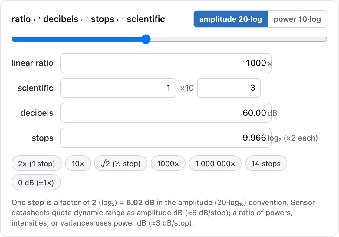
Figure 2.8.5(reproduced). A units converter for ratios (interactive). Decibels, photographic stops (log₂), a plain linear ratio, and scientific notation are four ways of writing one multiplicative factor. Type into any field, or drag the log-progression slider, and the others update to match; a toggle switches the decibel convention between amplitude ($20\log_{10}$, about 6 dB per stop, the convention sensor datasheets use for dynamic range) and power or energy ($10\log_{10}$, about 3 dB per stop, for ratios of intensities or variances). Preset chips jump to the common landmarks: one stop, ten-fold, a million-to-one, a full-frame sensor's roughly fourteen stops.
A standard-range display in good conditions (dim room, no glare) shows perhaps 1,000:1, about 10 stops, and much less in daylight, when reflected room light raises its black. Video projectors in a classroom can be as low as 10:1. A glossy print reflects roughly 100:1 to 250:1 if you avoid the reflection angle. Each number depends on the criterion used to define its dark end, which is why they should be compared with care.
Use a simplified linear observation model after black-level subtraction. The exposure factor $k_i$ includes shutter time, aperture transmission and calibrated gain; it converts scene radiance to the chosen signal units:
Each frame scales the same radiance, adds noise and clips at its recording limits. This approximation omits spatially varying optics, motion during exposure and nonlinear processing. Gain changes the signal units and noise model; it does not collect more photons.
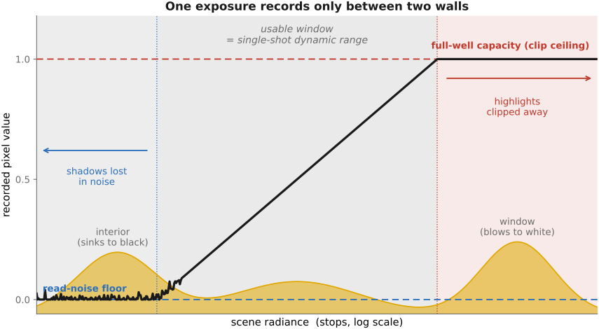
Figure 17.1.4(reproduced). One scene, one exposure, and the two walls of the single-shot dynamic range. A high-contrast scene (interior plus bright window) is shown with its radiance histogram laid against the photosite's response: highlights past the full-well capacity clip to a flat ceiling (the window blows to white), and shadows beneath the read-noise floor drown in noise (the interior sinks to black). The usable window between the two walls (the single-shot dynamic range) is shaded; the scene's true range overflows it on both ends. This is L2.46 drawn for one capture: dynamic range is the ratio of that ceiling to that floor.
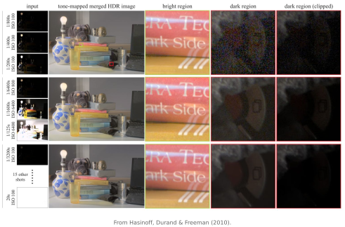
The principle of multiple-exposure high-dynamic-range photography is simple. Choose exposure factors with overlapping usable ranges, take photos, then merge into a floating-point radiance estimate. Its scale is usually relative unless an absolute radiometric calibration is supplied. Formats such as OpenEXR can preserve scene-linear values for later rendering (Chapter 8.11, File formats and compression).
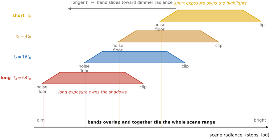
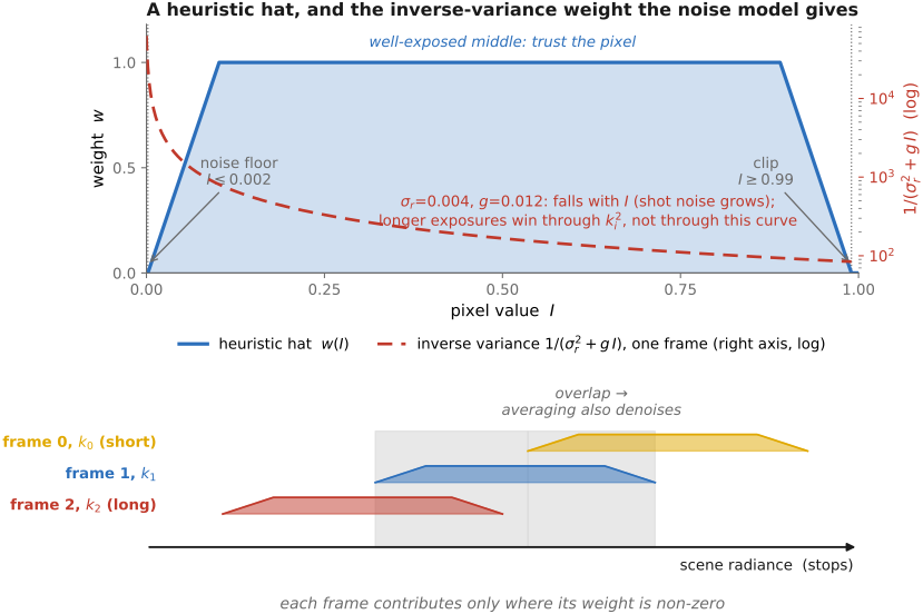
On a logarithmic radiance axis, changing exposure slides each frame's useful interval. One stop moves it by a factor of two. Overlap matters because neighboring exposures need common usable signal for calibration and a smooth change in which measurement is most precise. A gap leaves intensities that are clipped in one frame and poorly measured in the next. The merged floating-point values can exceed one; that is normal for a scene-linear representation whose scale is relative.
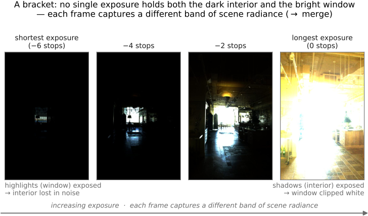
Figure 17.1.5(reproduced). A bracket tiles the radiance axis. The horizontal axis is scene radiance (log scale, in stops); each exposure $I_i$ in the bracket is drawn as a usable band (above its noise floor, below its clip ceiling), and increasing the shutter time $t_i$ slides the band leftward (toward dimmer radiance). A short exposure owns the highlights, a long one owns the shadows, and the bands overlap so that together they cover the full scene range. The merge keeps the reliable part of each band and stitches them into one radiance map spanning the whole axis.Figure 17.1.6(reproduced). The same idea on a real bracket: a dim interior with a blown-out window onto Boston harbor, a textbook high-dynamic-range scene. Four frames of a longer sequence, from the shortest exposure (the window and skyline are correctly exposed, but the room is lost in noise-black) to the longest (the room opens up, but the window clips to featureless white). No single frame holds both ends; each captures a different band of scene radiance, exactly the bands the previous figure drew, which is why the scene must be bracketed and merged.
The exposure factor $k_i$ can change in several ways, but each control changes something else as well. A useful capture sequence considers those side effects before choosing how widely to space its exposures.
For a conventional bracket, keep aperture, focus and gain fixed and vary shutter duration. This preserves the lens's focus blur and usually provides predictable exposure ratios. It also changes motion blur and capture timing, so the frames are not identical apart from brightness.
Under steady illumination and away from clipping, expected photon count is proportional to exposure duration. A longer exposure improves photon statistics but integrates more subject or camera motion and accumulates more dark current. Flickering light and rolling-shutter timing can violate a simple global exposure ratio.
Changing aperture changes depth of field, diffraction and often vignetting. Changing ISO changes gain and possibly input-referred read noise or saturation headroom, without changing the photons captured at fixed shutter and aperture. A neutral-density filter attenuates light, including flash, but its transmission and color should be calibrated. These controls can be useful in a designed capture sequence; they are not interchangeable with shutter duration.
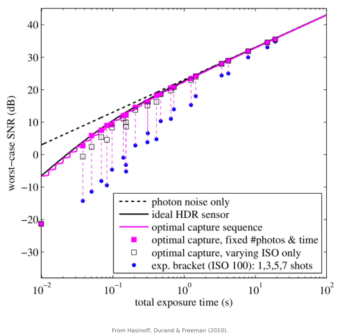
Set the shortest exposure to preserve important highlights and the longest to reach acceptable shadow SNR without excessive motion blur. Choose intermediate exposures with enough overlap for calibration and merging. Stop adding frames once they provide little useful coverage or noise reduction for their time cost.
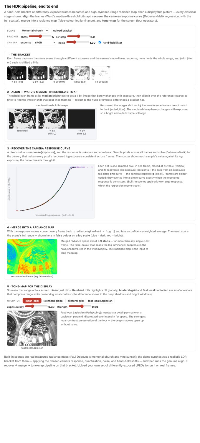
A tripod reduces camera motion but does not freeze subjects, foliage or illumination. Handheld brackets need registration; even tripod brackets need consistency checks. Ward's median-threshold bitmap (MTB) aligns differently exposed images using thresholded intensities and excludes values near the median (Ward 2003 (MTB)); Chapter 17.4, Ghosts and motion shows it at work. Clipping, noise and changing content can still corrupt the comparison.
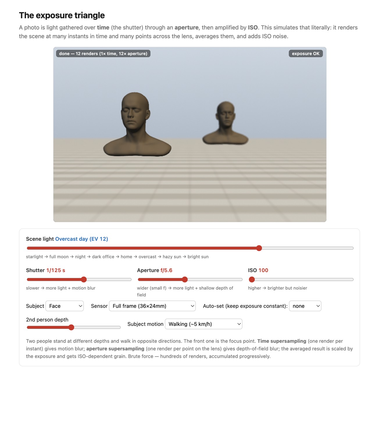
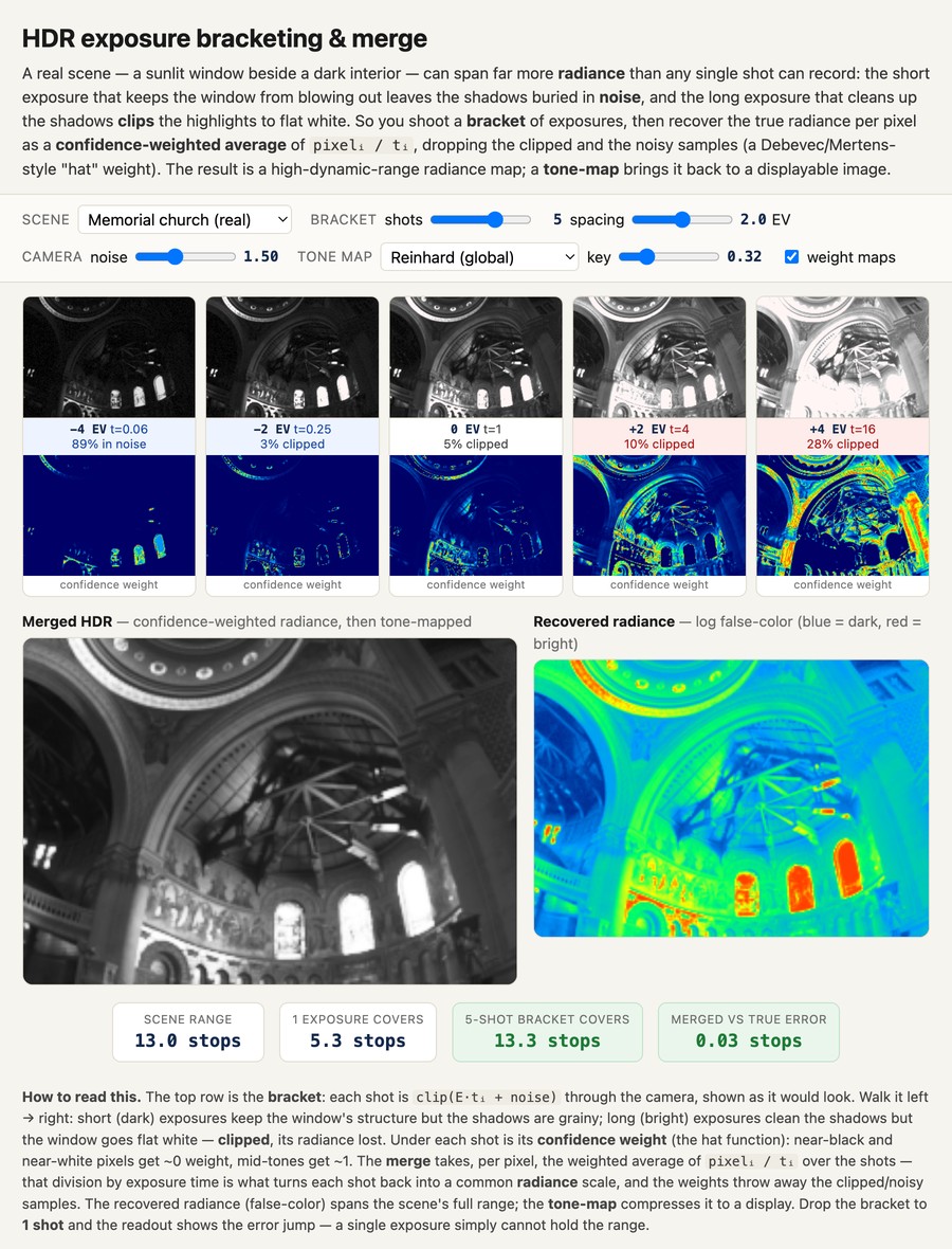
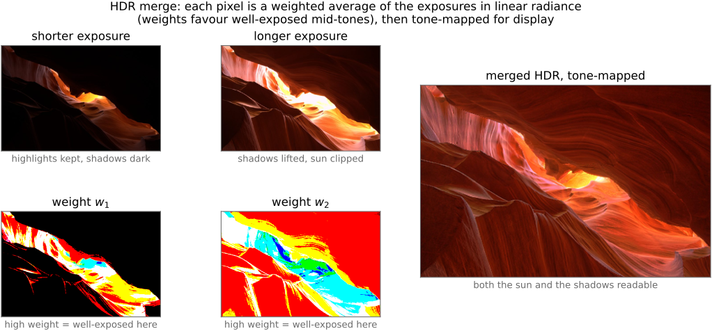
Figure 5.2.6(reproduced). Interactive: drive the three clean exposure knobs and watch each side effect appear. Hold the brightness fixed and trade one stop of shutter for a stop of aperture or ISO, and the picture's tone barely moves while its character changes: longer shutter brings motion blur, wider aperture (smaller f-number) shallower depth of field, higher ISO more noise. For bracketing, this is the figure's lesson made tangible: only shutter changes nothing but the exposure (so it is the knob you bracket with), while aperture would smear the focus across frames and ISO would amplify noise. (The fourth fallback knob, an ND filter, is the one this demo cannot show: it darkens the world but is not perfectly neutral, adds a color cast, and forces you to touch the camera.)Figure 17.1.7(reproduced). Interactive: why you bracket, and how the merge works. Pick a scene, either a real measured radiance map (Paul Debevec's classic memorial church, ~13 stops of bright stained glass over a dark nave, or his vine sunset) or a synthetic scene with an exactly-known true radiance, and the demo captures it as an EV bracket (sliders for shot count and spacing); each frame shows real highlight clipping and shadow noise, so no single exposure holds the whole scene. The demo then merges them, a confidence-weighted per-pixel average of $\text{pixel}_i/t_i$ that drops clipped and noisy samples (the Debevec/Mertens hat weight Debevec & Malik 1997), into an HDR radiance map, and a tone-curve slider maps it to display. Watch the per-shot weight maps, recover a blown highlight from the short exposure and a noisy shadow from the long one, and narrow the bracket to see the error return. (Real HDR maps courtesy Paul Debevec.)
Stops make the sequence easy to reason about: $1/1000$, $1/250$ and $1/60$ second form an approximately two-stop progression. The same exposure increase could be obtained by opening the aperture two stops, but then depth of field and the blur operator change. Flash gives another reason to distinguish controls. Within ordinary flash-sync operation, changing shutter duration mainly changes the continuous-light contribution; a neutral-density filter attenuates both ambient and flash light. The desired bracket must therefore account for which source the control actually changes.
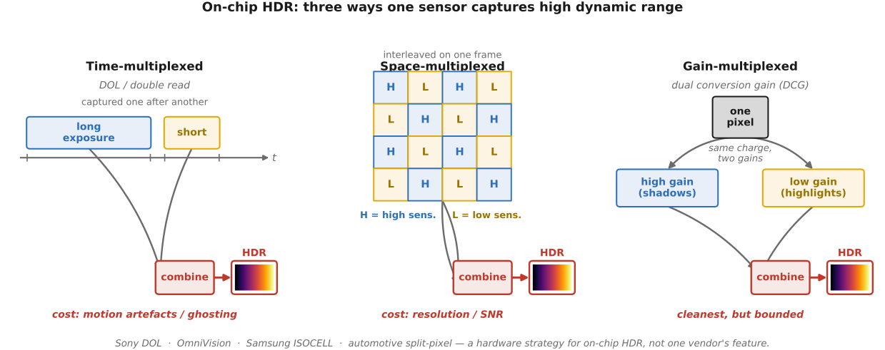
Sensors can combine measurements with different integration intervals, conversion gains or sensitivities into one delivered HDR frame. A single output frame does not necessarily mean all its measurements cover the same time interval. Check the sensor's acquisition and readout design (Part 34, Computational sensors).
Time multiplexing combines shorter and longer integrations. Digital-overlap HDR interleaves their readout; it should not be described as simply reading one unchanged exposure twice. Different integration windows can produce motion or illumination inconsistencies even when packaged as one output frame.
Gain multiplexing can read charge collected during a common integration through paths with different conversion gains. One path favors low input-referred read noise and another highlight capacity. This avoids the inter-exposure mismatch of a bracket when the integrations are shared. Ordinary selectable dual-conversion-gain operation does not by itself imply that both gains are delivered simultaneously.
Spatial multiplexing assigns different sensitivities or collection areas to neighboring sites or subpixels. Nayar and Mitsunaga's spatially varying exposure array reconstructs a wide-range image from such a pattern (Nayar & Mitsunaga 2000). The sampling and noise tradeoffs depend on the layout. Overflow-capacitor designs instead add charge storage; logarithmic or companding responses allocate output precision nonuniformly across intensity. None removes the need for calibration or a noise model.
Split-pixel sensors, common in automotive cameras, are a concrete spatial design. Each pixel holds a large photodiode and a small one. For the same light the small one collects far fewer electrons, so it saturates much later and records the highlights while the large one records the shadows, and the two are merged into one value per pixel. The motivating scene is a car leaving a tunnel: dark walls and daylight at the exit in one frame, with no time to bracket, plus LED signs and headlights driven by pulses that a short exposure can miss entirely. Because the small diode can integrate over a long window without saturating, it can record those pulses where a short exposure of the large diode would not. The two diodes differ in noise, response and color, so the merge needs its own calibration.
Compare integration timing, spatial sampling, read noise and saturation capacity separately. Shared integration avoids one source of ghosts, but does not eliminate motion blur or rolling-shutter distortion. A software burst adds repeated readout, computation and alignment costs.
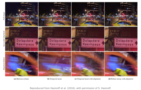
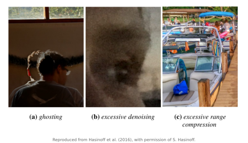
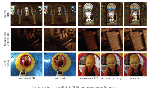
Figure 17.1.8(reproduced). On-chip ("direct") HDR sensors, organized by where they multiplex the dynamic range. Time-multiplexed (DOL "double read"): long and short reads of the same frame are combined; the schematic shows the two interleaved reads and a ghosted moving object flagging the motion artifact. Space-multiplexed (split-pixel large+small sub-photodiode, and SVE / assorted-pixels exposure mosaic): neighboring sites carry different sensitivities, single-shot but at a resolution/SNR cost. Gain-multiplexed (dual-conversion-gain): the same instant read at two readout gains: cleanest, but its added range is bounded. Each cell labels its cost (motion / resolution+SNR / bounded range), and a fourth panel contrasts the software HDR+ burst Hasinoff et al. 2016: maximal flexibility, paid in compute and alignment.
Two caveats: single-shot range, and where this is used⧉
First test a single raw file at the intended output size. Bracketing helps when it supplies cleaner shadows or unclipped highlights that the single capture lacks. Fill flash and graduated neutral-density filters can also reduce scene contrast at capture; dodging and burning change its rendering afterward.
These choices have photographic precedents. Le Gray combined negatives to retain sea and sky, while graduated neutral-density filters and fill flash change the contrast presented to the camera. Dodging, burning and the Zone System help control how recorded tones become a print; Chapter 18.9, High dynamic range in traditional photography, in the tone-mapping part, treats each of them.
Merging multiple exposures requires the conversion of pixel values into the same meaningful units proportional to scene radiance. Calibration establishes that relationship. When working with raw files, where the pixel values are linearly related to radiance, only pairwise ratios are needed. In the general case, the non-linear response curve from radiance to pixels must be calibrated. The unknown scene can help calibrate the camera because each scene point appears at several exposures. We assume the images in a bracket are pixel-aligned and the scene does not contain movement. The model $I_i=f(k_iL)$ assumes a fixed pointwise response shared across frames, where $k_i$ characterizes the exposure for frame $i$. In the general case $f$ must be calibrated. We assume $I_i$ values have been black-level corrected (recall that some cameras add a constant offset to measure the negative component of readout noise, Chapter 2.8, Noise, signal-to-noise ratio and dynamic range). Throughout, $I_{p,i}$ is the value of pixel $p$ in frame $i$, $L_p$ the radiance at that pixel, and $w(I)$ a reliability weight that is zero for clipped values and small near the noise floor.
In the linear case, $f$ is simply a global multiplication factor and the problem boils down to recovering the $k_i$ exposure factors up to a multiplicative factor. But even for linear RAW files, linearity breaks down for dark values, and especially for bright ones. We call a pixel reliable if it is not too dark and not too saturated (between $\epsilon_0$ and $1-\epsilon_1$ in normalized pixel values). For exposure ratio estimation, the values of the thresholds are not critical and anything significantly above the read-noise level will do.
For linear, black-level-corrected reliable observations, $I_{p,i}=k_iL_p$ in the noiseless unsaturated model. At a pixel that is reliable in two images, the radiance cancels:
Pairwise ratios recover relative exposure factors, but small denominators and noisy correspondences can bias them. Use many reliable pixels and validate residuals; jointly fitting exposure scales can avoid drift from chaining. Metadata supplies a useful initial estimate and can be accurate enough for some cameras. The image only determines relative radiance without an absolute calibration.
To avoid statistics over ratios, which is always dangerous when denominators can be close to zero, you can use a linear regression where you fit the scalar $\frac{k_i}{k_j}$ according to the model
$$ I_{p,i} = \frac{k_i}{k_j} I_{p,j} $$
which naturally weights the more reliable evidence from larger pixel values higher. But in practice, the median works fine, especially if you exclude ratios with low denominators.
If pixels exhibit inconsistent values between normalized frames, check black level, response, timing, illumination and registration before merging.
Validate exposure factors
Metadata records nominal capture settings. Check them against unsaturated, registered image regions when radiometric accuracy matters (Burggraaff et al. 2019). Pixel-based calibration also has failure modes: motion, flickering light, noise and local processing can make a single global ratio inappropriate.
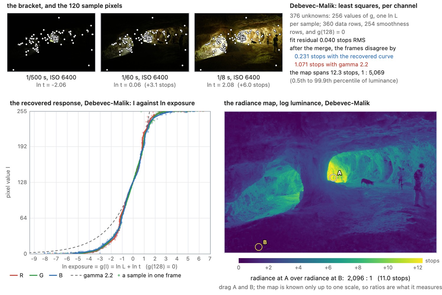
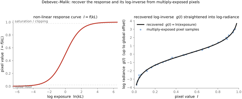
In the non-linear case, we need to recover the response curve. Real cameras (and film, and JPEG) apply a non-linear response $f$, such as a gamma, a tone curve, or a film characteristic, including the beauty curve that gives a camera its look (Why scene-linear looks dull, in Part 8, Basic image processing and ISP). Then $I_i = f(k_i L)$, and you must recover $f$ (equivalently its log-inverse $g = \ln f^{-1}$) before you can merge. The trick of Debevec and Malik (1997) is that a pixel imaged at several exposures gives several $(I_{p,i}, t_i)$ pairs that all constrain the same radiance $L_p$, and that over-determination pins down the curve. Here aperture and calibrated gain are fixed, so $k_i$ is the shutter time $t_i$ times a common scale, which is absorbed into $L_p$. Working in the log domain, each observation says
$$ g(I_{p,i}) = \ln L_p + \ln t_i. $$
The unknowns are the curve $g(\cdot)$, one value per possible pixel level, say 256 of them, and one $\ln L_p$ per pixel. Stack one such equation per pixel per exposure and you have a linear least-squares system in $g$ and the $\ln L_p$'s, solved jointly, exactly the kind of inverse problem of Chapter 6.7, Image formation as a linear system. Two riders make it well-behaved: a smoothness penalty on $g''$ (a real response curve is smooth, not jagged), and the same reliability weight $w(I)$ we will use in the merge, down-weighting samples near the clip and near the noise floor. The recovered curve is fixed only up to one additive constant, again the global scale (Figure 17.2.2).
With sample pixel $p$ and frame $i$, one explicit fit is
Here $\ell_p=\ln L_p$, the second sum runs over the possible pixel values $I$, $\Delta^2$ is a discrete second difference, and $I_{\rm mid}$ is a mid-range value whose $g$ is fixed. Fixing one curve value removes the additive-scale ambiguity. The written weights multiply residuals before squaring; using weights outside the square is a different convention. Smoothness alone does not enforce a monotone response. Check the recovered curve and held-out exposure residuals.
The system is small. Each $\ell_p$ appears only in its own sample's rows, so it can be eliminated exactly, leaving a symmetric 255 by 255 system for $g$ per channel that solves in milliseconds (Figure 17.2.1). Run it on camera JPEGs and try three things. Set the weight to flat, and the clipped samples at 0 and 255 bend the ends of the curve. Lower $\lambda$ and the curve follows the noise; raise it and it can no longer turn at the toe. Merge with an assumed gamma of 2.2 instead of the recovered curve, and the frames of a bracket disagree about a pixel's radiance by about a stop, against a few tenths of a stop with the curve.
Figure 17.2.1(reproduced). Debevec and Malik, and Mitsunaga and Nayar, calibration on camera JPEGs (interactive). Top: a bracket of three JPEGs with shutter time and ISO from EXIF, and the sample pixels, drawn at random or one per band of intensity from flat neighborhoods. Left: the recovered log-inverse response $g(I)$ for R, G and B, solved per channel by least squares with the smoothness weight $\lambda$ and the weighting $w(I)$ chosen below the figure; each sample's observations sit at $\ln L_p + \ln t_i$, and the dashed curve is a gamma of 2.2 anchored at the same code value. Right: the bracket merged with the recovered curve, or with the gamma for comparison, into a radiance map shown as false-color log luminance or tone-mapped with global Reinhard; drag the probes A and B to read a radiance ratio. The readout gives the fit residual and how far the frames still disagree after the merge. The method control switches to Mitsunaga and Nayar's self-calibration Mitsunaga & Nayar 1999: a polynomial of degree $D$ (set by hand, or chosen on held-out pixels) fitted together with the exposure ratios, which can be started off EXIF; the panel at top right then plots the ratios and the error at each iteration, and the curve is drawn as $\ln f^{-1}(I/255) - \ln f^{-1}(128/255)$ so it shares the axes of $g$: the unknown scale of $f^{-1}$, which $f^{-1}(1) = 1$ fixes, is the same unknown as the constant in $g$, which $g(128) = 0$ fixes. Either method's curve can be overlaid on the other's. Where the camera changed ISO within a bracket, $t_i$ is shutter time times ISO/100. You can load your own bracket; exposure times are read from EXIF and can be edited. Photographs by Frédo Durand, the camera's own JPEGs (Sony α1 II and α7R V).
Mitsunaga and Nayar (1999) assume even less. They model the response as a low-order polynomial and recover it, together with the unknown exposure ratios, by radiometric self-calibration, so you need not even trust the EXIF exposure ratios. The spirit is identical: pixels seen at multiple exposures over-determine the curve, so fit a smooth response to them. (Mann & Picard 1995's "comparametric," or Wyckoff, work is the earlier multiple-exposure precursor to both.)
The figure runs their method as a second option on the same samples. Their model is the inverse response itself rather than its logarithm $g$: a polynomial of degree $D$, $f^{-1}(I) = \sum_{n=0}^{D} c_n I^n$, on pixel values normalized to $[0,1]$, with $f^{-1}(1) = 1$. Two steps alternate: with the exposure ratios $k_i/k_{i+1}$ of consecutive frames fixed, every pixel seen in both gives a linear equation $f^{-1}(I_{p,i}) = (k_i/k_{i+1})\, f^{-1}(I_{p,i+1})$ in the $c_n$, solved by least squares; with the curve fixed, each ratio is re-estimated as the average of $f^{-1}(I_{p,i})/f^{-1}(I_{p,i+1})$. Start the ratios a stop off EXIF, alternately up and down, and the iteration brings them back to within a few tenths of a stop. Start them all off the same way and it cannot. If $f^{-1}$ and the ratios $k_i/k_{i+1}$ explain the images, so do $(f^{-1})^{\gamma}$ and $(k_i/k_{i+1})^{\gamma}$ for any exponent $\gamma$, so the pictures fix the ratios only relative to one another, as Grossberg and Nayar showed Grossberg & Nayar 2003, and the polynomial model pins $\gamma$ only weakly. Run exactly as published on these JPEGs, the iteration drifts along that family, so the figure holds the bracket's total span in stops at its starting value, which removes that one direction and nothing else.
Joint fitting uses many observations while imposing a smooth response. It still requires sufficient exposure overlap and a suitable observation model. Debevec–Malik's conventional intensity weights are reliability heuristics, not automatically the inverse variances of log-transformed noise.
The log-domain estimate in Debevec–Malik is a weighted average of log exposures. Exponentiating it gives a geometric mean of radiance estimates, which differs from a linear-light arithmetic mean. Both can be useful under their respective error models; neither justifies averaging gamma-encoded values as radiance.
Figure 17.2.2(reproduced). The recovered camera response (Debevec–Malik). Left: the camera's non-linear response curve $I = f(kL)$ (pixel value against log exposure), an S-shaped film/JPEG curve. Right: its log-inverse $g(I) = \ln(kL)$, recovered by least squares from pixels seen at many exposures and straightened into log-radiance. Faint clusters of sample points (one cluster per pixel, spread across exposures and shifted by $\ln t_i$) are shown pinning the curve down, up to one global vertical offset; a smoothness penalty keeps $g$ from wiggling between samples.
With calibration and combination both in hand, run the whole pipeline end to end, once, on one bracket: alignment, response recovery, merge, and (a preview of) tone mapping in a single interactive (Figure 17.2.3).
Figure 17.2.3(reproduced). The HDR pipeline, end to end (interactive). A hand-held bracket is taken through every classical stage on one screen: (1) the differently-exposed frames, each shifted a little by hand tremor; (2) Ward's median-threshold-bitmap alignment, which thresholds each frame at its median into an exposure-invariant 1-bit image and slides it coarse-to-fine to recover the integer shift; (3) Debevec–Malik response recovery, with the full scatter of (value, log-exposure) samples from every frame falling onto the single recovered curve $g$; (4) the merge into a radiance map, shown in false color on a log scale; and (5) tone mapping to the display, switchable between linear (clip), Reinhard global Reinhard et al. 2002, bilateral-grid Chen et al. 2007, and fast local Laplacian Aubry et al. 2014 so the global-vs-local difference is visible in the windows and shadows. Built-in scenes are real radiance maps (Debevec's memorial and vine sunset) from which a realistic bracket is synthesized; you can also upload your own exposures. The tone-mapping stage is a preview; its operators are developed in Part 18, Tone mapping and display and Chapter 10.1, Bilateral filtering.
Calibration puts the exposures into common units. The next decision is how much to trust each estimate at each location. We start with a simple method based on thresholds. But we then observe that long exposures can supply precise shadows and clipped highlights at the same time, so a more advanced merge must combine both measurement values and their reliability.
We work with registered, black-level-corrected linear values $I_i$ and calibrated exposure factors $k_i$. We divide by $k_i$ to put the observations in common relative-radiance units, then combine the valid estimates. For encoded inputs, we first invert the appropriate response.
Validity masks reject saturated, defective or unregistered samples. Noise weights reduce the influence of uncertain measurements. We choose clipping margins in the input's calibrated units; thresholds such as 0.99 or 0.002 are not universal. Very dark samples can still provide information when their noise is modeled. We avoid selecting on noisy intensity more aggressively than necessary, since this can bias the merge.
We let $w_i$ include both validity and reliability. The linear-light merge is
In words, the estimated radiance is the reliability-weighted mean of the rescaled observations. In code this is one pass per pixel over the bracket: divide out each exposure factor, accumulate by reliability, normalize:
Algorithm 1
for each pixel p:
num, den = 0, 0for each exposure i:
if valid(i, p):
q = linear_value(i, p) / exposure_factor[i]
w = radiance_weight(i, p)
num += w * q
den += w
if den > 0:
L[p], measured[p] = num / den, True
else:
L[p], measured[p] = flagged_fallback(p), False
For a calibrated nonlinear response, Debevec–Malik Debevec & Malik 1997 instead combines log-radiance estimates:
Exponentiation produces a weighted geometric mean, not the preceding arithmetic mean. The error model and weighting should match the domain. Multiple independent, equally precise observations reduce standard deviation by $1/\sqrt N$; unequal weights, correlations and data-dependent selection require the more general variance calculation (Chapter 13.2, Denoising by averaging).
If every exposure clips, the shortest exposure supplies the strongest lower bound on radiance. If all are too noisy, the longest usable exposure is usually the best fallback at fixed gain, provided motion and defects do not invalidate it. We keep an uncertainty or validity flag, since neither case supplies a reliable point estimate. With variable gain, we select by calibrated radiance-domain uncertainty rather than by exposure duration alone.
Chapter 18.4, Exposure fusion directly blends rendered inputs using appearance weights. It is useful when a finished picture is the objective; its output is not a calibrated radiance measurement.
Figure 17.3.1(reproduced). The reliability weight $w(I)$ as a function of pixel value. The weight is zero at the clipped end (e.g. $I \ge 0.99$) and zero at the dark, noisy end (e.g. $I \le 0.002$), rising to a plateau in the well-exposed middle, a hat shape. A dashed overlay shows the SNR-optimal version of the weight, skewed toward the brighter, less-noisy samples rather than symmetric. Below, a sketch of three bracket frames shows each contributing only over the band where its weight is non-zero, with overlap regions (where averaging also denoises) shaded.Figure 17.3.2(reproduced). The merge on a real bracket (Antelope Canyon). A shorter exposure keeps the bright sunlit slot but buries the rock in noise-dark shadow; a longer exposure lifts the shadows but clips the sun. Each frame's weight map (rainbow, bright means high weight) marks where it is well-exposed, neither clipped nor noisy. The reliability-weighted average in linear radiance keeps the good band from each, and the float radiance map is then tone-mapped for display, so both the sun and the deep shadows read at once.
A binary validity mask can retain several exposures at once. Among the valid estimates, inverse-variance weights account for unequal precision instead of treating all samples equally.
For two independent unbiased estimates $x,y$ with variances $\sigma_x^2,\sigma_y^2$, we write $\hat L=\beta x+(1-\beta)y$. Minimizing $\beta^2\sigma_x^2+(1-\beta)^2\sigma_y^2$ gives:
Under independence and known positive variances, the minimum-variance linear unbiased estimate weights each observation by inverse variance. Here $\sigma_i^2$ must denote variance after exposure normalization, in radiance units:
$$ \hat L = \frac{\sum_i (I_i/k_i)\,/\,\sigma_i^2}{\sum_i 1/\sigma_i^2}, $$
The preceding result applies to independent estimates with fixed known variances. Saturation and uncertain calibration need separate treatment.
To make those weights concrete, we plug in the camera's noise model. The per-pixel variance is dominated by two terms: photon (shot) noise, whose variance is proportional to the signal and so dominates in the highlights, and read noise, whose variance is constant and so dominates in the shadows:
$$ \sigma^2(x) = a\,x + \sigma_\text{read}^2, $$
where $a$ and $\sigma_\text{read}$ depend on the camera and the ISO. We can calibrate it by shooting repeated frames and measuring the variance across the stack, or derive it on paper. Either way, the merge weights are no longer a hand-drawn hat; they come from the physics of the sensor.
If linear signal $I_i$ has conditional variance $a_i k_iL+b_i$, then the normalized estimate has
At common gain with shot noise alone, the relative weights are proportional to $k_i$ for each valid frame. With read noise, the weights generally also depend on scene intensity. We handle that dependence with a pilot radiance estimate or an appropriate likelihood. For correlated measurements, the covariance matrix replaces independent inverse variances. Clipping and data-dependent weights also limit the unbiased-estimator interpretation.
We can measure what each choice of weights does to the noise of the merge on a simulated bracket (Figure 17.3.4). Weights proportional to $k_i$ match the hat almost everywhere and do much better just below the level where a frame clips, where the hat discounts the best sample. In the shadows, where read noise dominates, they trust a short frame too much, and the hat does slightly better there. Only the inverse variance is never worse than the others, and weighting by $1/k_i$, which favors the short frames, is clearly worse than all of them.
Figure 17.3.4(reproduced). Merge weights against the noise of the merged radiance, on a bracket simulated from a radiance map of an office. Each frame is $I_i=\min(1,\,k_iL+n_i)$, with Gaussian noise of variance $a\,k_iL+\sigma_\text{read}^2$ standing in for photon and read noise, drawn once with a fixed seed. Stage 1 plots the SNR of each frame's own estimate $I_i/k_i$ against $\log_2 L$. The next stages merge the frames with binary validity, the Debevec and Malik hat, $w_i\propto k_i$, and the inverse variance $w_i\propto 1/v_i$; all but the last also drop samples below $I_i=0.002$. Lines are the closed form $\operatorname{Var}(\hat L)=\sum_i w_i^2v_i/(\sum_i w_i)^2$, dots the error measured against the noiseless radiance, and the two agree. The weights are evaluated at the noiseless radiance, as a perfect pilot estimate would give them. At the default camera, binary validity loses up to 17 dB where a short frame barely clears the floor, since it trusts that frame as much as a long one. The hat and $w_i\propto k_i$ agree except just below where a frame clips, where the hat discounts the best sample and loses up to 7 dB. In the shadows, read noise makes $w_i\propto k_i$ trust a short frame too much, and there the hat does a little better (15.9 against 15.3 dB measured in the crop); only the inverse variance is best everywhere. Turned on, $w_i\propto 1/k_i$ runs the weighting the wrong way: the crop falls to 6.8 dB, below binary validity's 10.7. Radiance map: Byong Mok Oh. Interactive: step through the stages; click or drag the box on the scene to move the crop; change the number of frames, their spacing, the shortest exposure, the photon gain $a$, the read noise $\sigma_\text{read}$ or the radiance map. Lowering $\sigma_\text{read}$ closes most of the gap between $w_i\propto k_i$ and the inverse variance.
Hasinoff, Durand and Freeman optimize the shutter/ISO sequence for worst-case SNR over a specified brightness range and time budget, using a calibrated camera noise model (Hasinoff et al. 2010). Higher gain can reduce the contribution of downstream read noise on some sensors, at the cost of saturation headroom. The optimum is camera- and scene-dependent; it does not imply a general preference for short, high-ISO exposures. Granados and colleagues develop related noise-aware merging (Granados et al. 2010).
Figure 17.3.5(reproduced). The strategy on a real scene: a high-contrast church interior in Nancy. A bracket merged with the noise-optimal capture set recovers both the sunlit windows and the deep shadowed nave in one radiance map, the kind of interior that overflows any single exposure on both ends. What to notice is that the shadows come back clean rather than grainy: the gain in worst-case SNR is exactly what keeps the darkest regions usable Hasinoff et al. 2010.Figure 17.3.6(reproduced). A second real-scene result of the noise-optimal capture strategy. A high-dynamic-range scene shot with the SNR-optimal shutter-and-ISO set and merged, shown against what naive bracketing yields under the same time budget; the optimal capture holds detail across the range with visibly cleaner shadows. The theory transfers to practice: choosing which exposures to shoot, beyond how to weight them, measurably improves the merged result Hasinoff et al. 2010.
The fixed-time capture question also matters for bursts: additional frames incur readout and alignment costs. Chapter 17.6, HDR+ and burst imaging on phones uses a different capture design, retaining short exposures for highlights and motion while combining them for noise reduction.
Figure 17.3.7(reproduced). The SNR-optimal exposure set (Hasinoff–Durand–Freeman). SNR (in dB) is plotted against log scene brightness for three strategies: standard bracketing at ISO 100, the SNR-optimal high-ISO short-exposure set, and the ideal HDR sensor as an upper bound. The optimal set lifts the worst-case (darkest-region) SNR by roughly 12 dB over naive bracketing and tracks close to the ideal curve across the range, the counter-intuitive result of using higher ISO and shorter exposures once the noise model is taken seriously.Figure 17.3.8(reproduced). The same argument in the authors' own plot, beside our reproduction above. Worst-case SNR is traced against exposure time for each strategy under a fixed time budget: naive ISO-100 bracketing sits well below the SNR-optimal set that favors higher ISO and shorter shutters, which in turn hugs the bound of an ideal HDR sensor. Seeing the published figure makes the claim concrete: once the full photon-plus-read noise model is taken seriously, fewer, shorter, higher-ISO frames win, lifting the darkest-region SNR by roughly 12 dB Hasinoff et al. 2010.
Calibrated HDR scenes for tone-mapping evaluation; Google's RAW burst set behind HDR+ Hasinoff et al. 2016. <http://markfairchild.org/HDR.html> · <https://hdrplusdata.org>. See the Chapter 45.16, Datasets appendix.
The units of the weight are easiest to see with two exposure times. A long exposure records more photons, but its raw variance is also larger in the shot-noise regime. Dividing each measurement by its exposure time puts both on a radiance scale. The long exposure then has smaller variance on that common scale, because the exposure normalization divides its variance by the square of the time. Weighting raw values by their unnormalized variance would answer the wrong question.
With shot noise alone, the precision of an unclipped radiance estimate grows in proportion to exposure time. Read noise adds a term whose radiance variance decreases with the square of exposure time, making long captures especially useful where that term matters. Clipping removes their usefulness at bright pixels. This is how one frame can be valuable in the shadows and unusable in the highlights without changing the weighting principle.
The capture optimization asks a different question from choosing merge weights. Suppose the total capture time is fixed. Spending most of it on a long exposure gives dark regions more photons, but can leave bright regions clipped in that frame. Dividing it among short exposures provides repeated highlight measurements but incurs read noise repeatedly. Changing gain can alter the contribution of downstream electronics as well as the available headroom. For each candidate sequence, we predict the merged SNR as a function of scene brightness; the objective used by Hasinoff, Durand and Freeman improves the worst part of that curve over a specified range Hasinoff et al. 2010. The figure's comparison should be read as a result for its camera model and budget, rather than as a universal ISO prescription.
The published capture example makes the role of gain concrete. Under a budget of at most three photographs and 0.25 seconds of exposure, the paper's Canon 1D Mark III model compares an ISO-100 bracket of $1/100$, $1/25$ and $1/6$ second with an optimized ISO-3200 sequence of $1/3200$, $1/125$ and $1/5$ second. Its plotted worst-case SNR improves by about 12 dB (project poster). The longest optimized exposure is actually longer than the longest bracket exposure. The result comes from allocating the whole sequence under the sensor's noise and saturation model, not from a rule that increasing ISO and shortening every exposure improves photographs.
A handheld camera faces both limited light collection and motion. Longer exposures improve photon statistics but can blur, while shorter exposures require more frames to collect the same total light and pay read noise repeatedly. Capture policy therefore depends on scene motion, illumination and sensor characteristics.
HDR+ uses equal-exposure raw frames to reduce noise while preserving the highlight range of its chosen short exposure. It improves usable shadow range; it does not extend the saturation threshold by measuring brighter highlights at a second exposure. This differs from a conventional bracket, whose frames cover different radiance intervals.
An exposure chosen to protect highlights may leave noisy shadows. Independent repeated measurements can reduce that uncertainty, whereas a highlight clipped in every frame remains only bounded from below. In a normalized noiseless model, protecting a chosen maximum radiance requires
$$ k\,L_{\max} < 1, $$
Noise and uncertain metering require a margin; transient or deliberately unprotected highlights may still clip. Extra frames do not guarantee usable shadows under a fixed time budget. Choose which highlights matter rather than imposing an unconditional no-clipping rule.
💡 Big lesson ((L13.1) · Capture the full set, decide later)
The burst is L13.1 on a phone: capture many identical frames now and defer the noise-versus-range tradeoff to a downstream merge. (L13.1 first appears in this part's introduction; the light-field/plenoptic camera (Part 33, Computational optics and coded imaging) is the same idea for the focus/viewpoint axis, the special case.)
Noise-optimal bracket design (Hasinoff et al. 2010) and HDR+ both account for noise, but they solve different capture problems. A uniform short burst is not the universal optimum of the earlier shutter/ISO optimization. Motion, latency and available buffering also influence the deployed design.
Figure 17.6.2(reproduced). Burst, not bracket. Left, classic HDR bracket: a few frames at different exposures (short for highlights, long for shadows); demands a static scene and a steady mount, and the long frame blurs while moving subjects ghost between the differently-exposed frames. Right, HDR+ burst: many frames at one identical, short, deliberately under-exposed setting; hand-held, motion frozen, every frame the same so alignment is easy, and the noise of the short exposure is beaten down $1/\sqrt N$ by merging. The bracket varies exposure across few frames; the burst holds exposure fixed across many.Figure 17.6.3(reproduced). The irreversibility asymmetry. Top, a single "correctly" exposed frame: the bright window clips to flat white; the detail above the full-well ceiling is destroyed and unrecoverable. Bottom, an under-exposed burst: the same window stays below clipping in every frame, so its detail survives, while the now-darker, noisier shadows are cleaned up $1/\sqrt N$ after the merge. A clipped highlight is gone forever; a noisy shadow is only noisy, so bias the exposure down ($k\,L_{\max}<1$) and recover the shadows by computation.
The paper's own teaser shows what the underexposed burst buys at the hardest extreme: a near-dark, hand-held portrait.
Figure 17.6.4(reproduced). HDR+ in the dark. A near-black, hand-held selfie that a single short frame renders as noisy murk (left) becomes a clean, well-exposed portrait (right) after a burst of identical underexposed raws is aligned and merged; the eye crops show grain beaten down and detail restored, with no motion blur. The whole multiple-exposure part, shipped to a phone (Hasinoff et al. 2016).
Compare a shadow patch with a lamp that is saturated in every frame. The shadow measurements can vary around a useful underlying signal, so combining independent observations can make that signal more precise. The clipped lamp values do not vary with how far the true signal exceeded the ceiling; averaging the ceiling repeatedly supplies no measurement of that excess. This asymmetry motivates reserving highlight headroom and paying some of the cost as shadow noise. It does not make arbitrarily short exposures desirable: read noise, total capture time, rejected frames, and values lost below the usable floor still constrain what the burst can recover.
Choose a reference, estimate local alignment and combine consistent raw samples. Maintain CFA phase, black-level and gain conventions. After raw merging, demosaic and render the result. The exact interpolation and alignment precision depend on the implementation; the original HDR+ and later burst-super-resolution pipelines should not be conflated.
Raw merging retains access to sensor-domain measurements and a calibrated noise model. Interpolation and merging can still introduce correlations. Joint reconstruction or a suitably modeled RGB pipeline are alternatives; pre-demosaic processing is a design choice rather than a universal optimality result.
A simplified spatial-weighted model illustrates exposure normalization, although the actual HDR+ merge operates on tile transforms:
HDR+ uses a transform-domain merge on aligned tiles, with shrinkage informed by estimated noise and differences from the reference. This differs from simply assigning a per-pixel inverse-variance weight. Large inconsistencies reduce temporal averaging; a reference fallback sacrifices noise reduction to limit motion artifacts. Equal averaging provides a useful independent-noise reference case:
This approximation assumes equal noise and independent, correctly registered samples. Rejection, adaptive filtering and correlated errors change it.
Local alignment handles some motion that a global transform misses. Occlusions and varying exposure blur remain difficult, so the merge needs confidence and fallback even after alignment. For a merged image, inspect both detail and the spatial variation in noise rather than reporting burst length as the number of useful samples everywhere.
Figure 17.6.5(reproduced). The HDR+ flow. Left to right: a burst of $N$ identical under-exposed raws → pick a sharp reference frame → align every other frame to it (tile-based, sub-pixel) → robust merge in raw (Wiener-style; reject mis-aligned or moving tiles) → a single denoised, high-DR raw → demosaic → tone-map and finish → JPEG. The decisive choice is that the merge, which does denoising and HDR together, happens in raw, before demosaicking.
The original paper draws the same flow on a real scene, and shows both why alignment is decisive and how the finished pipeline compares to a conventional ISP.
Figure 17.6.6(reproduced). The HDR+ pipeline as the authors drew it. From a live viewfinder fed by the hardware ISP, the shutter press grabs a burst of raw frames at one chosen exposure-and-gain; these are aligned and merged at full resolution, then run through white balance, demosaic and chroma denoise, a local tone map (exposure fusion Mertens et al. (exposure fusion)), dehaze and global tone map, and a final sharpen and saturation pass. The decisive step, align-and-merge, sits before demosaicking, so denoising and HDR happen together on the raw signal (Hasinoff et al. 2016).Figure 17.6.7(reproduced). Why alignment decides the result, on a night street. The same moving scene merged four ways: a single reference frame (noisy), a naive temporal mean (motion smears the sign and the passing vehicle into a ghost), the mean with alignment (the static sign sharpens, but residual motion still ghosts), and the robust merge with alignment (the sign is crisp and the moving vehicle is handled without a double image). Alignment plus the outlier-rejecting weight is exactly what turns a helpful average into a clean result (Hasinoff et al. 2016).Figure 17.6.8(reproduced). Three ways a burst merge goes wrong, named. (a) Ghosting, a moving subject left a double image where the merge trusted misaligned frames; (b) excessive denoising, over-aggressive averaging smeared away real texture into a waxy blur; (c) excessive range compression, the tone map pushed local contrast flat and hazy. The failure gallery that the robust weight, a light hand on denoising, and a restrained tone curve each exist to avoid (Hasinoff et al. 2016).Figure 17.6.9(reproduced). Conventional ISP versus HDR+, across hard scenes. A dim church interior, a low-light living room, and a moving child are each shown as a conventional single-frame ISP result beside the HDR+ result (and, for the child, the cost of not merging). The burst pipeline holds highlights, cleans shadows, and freezes motion where the conventional pipeline leaves noise, blur, or clipping (Hasinoff et al. 2016).
Tile alignment makes a local motion approximation. A tile on a stationary wall and a tile on a moving arm can choose different displacements, whereas one global translation must compromise between them. But a tile straddling the arm boundary contains two motions. No single displacement aligns both, and a newly revealed background patch has no corresponding foreground sample to average. The robust merge handles some of these failures by reducing inconsistent contributions. Where fewer observations survive, more noise remains. The alignment and merge therefore need to be understood together: locally different noise levels can be the visible consequence of preserving moving structure.
Photographers were fighting dynamic range more than a century before anyone merged a bracket in software. The scene has always had more range than the print can show, and for most of that history it also had more range than the negative could record. What they did about it maps closely onto the capture methods of Part 17, High dynamic range capture and onto the tone-mapping chapters of this part: combining several exposures, measuring the scene and deciding where each tone should land, and compressing large-scale contrast while keeping local detail. Knowing the craft makes the algorithms easier to read, and several of their failure modes, the halo above all, were met in the darkroom first.
This chapter follows the photographer through the three places a traditional workflow can intervene: in front of the camera, at capture and development, and at printing. Chapter 5.5, Developing and editing a photograph describes the darkroom as a whole; here the focus is on range.
A black-and-white negative-positive process has two stages with very different ranges. A negative can record a wide range of scene luminance, commonly ten stops or more with care, because its response rolls off gradually at both ends. A print on paper reflects light, and its range runs from the deepest black the paper can hold to the white of the paper base: a density range of about 2 on glossy paper, a ratio of about 100:1 or seven stops, and less on matte paper. The print cannot show what the negative holds, so every print is already a tone mapping, whether the printer thinks of it that way or not. Color slide film is the harder case: the transparency is the final image, it records only five or six stops, and there is no printing stage in which to rescue anything.
That gives three moments for control, each with its own tools:
Before the shutter: change the scene. Add light to the shadows, subdue the highlights, or wait for light whose range the process can hold.
At capture and development: change what reaches the film and how the film responds. Filters, exposure placement and development time decide which scene luminances end up as usable densities.
At printing: change how densities become print tones. Paper contrast, local exposure with dodging and burning, and masks decide where each part of the negative lands on the paper.
All three moments can be tried in a simulated darkroom that starts from a high-dynamic-range scene (Figure 5.5.2).
Figure 5.5.2(reproduced). A simulated black-and-white darkroom, from an HDR scene or your own .hdr file: expose the negative with a filter, a graduated ND and a zone placement; develop it from N−2 to N+2 on its characteristic curve; print it under an enlarger on graded paper, dodging, burning and sandwiching an unsharp mask. Each of this chapter's three moments is one of its tabs. The film, developer and paper responses are models.
The first photographers had a harsher problem than a short print range. Wet collodion, the standard glass-plate process from the 1850s, was sensitive almost only to blue and ultraviolet light. A sky, rich in blue, recorded far more strongly than a landscape or a sea of the same apparent brightness, so an exposure long enough for the land left the sky as a featureless, overexposed white. Painted-in or blank skies were common in landscape photographs of the period.
Gustave Le Gray's seascapes of 1856 to 1858, taken on the Normandy coast and at Sète on the Mediterranean, answered this in two ways. Some were single exposures made in favorable light, with short exposures that held the sky and let the sea go dark. Others combined two negatives: one exposed for the sea, one for the sky, printed one after the other onto the same sheet with the horizon as the join. The horizon is a gift to this method, a nearly straight line where the two exposures can meet without an obvious seam, and Le Gray used the same sky negative with more than one foreground (Getty exhibition). The prints were admired in their day partly because viewers believed they showed sea and sky together as the eye saw them, which a single collodion plate could not (Figure 18.9.1).
Figure 18.9.1(reproduced). Gustave Le Gray, The Great Wave, Sète, 1857, albumen print from glass negatives. The breaking wave and the clouds are both held, which a single collodion exposure of the period could not do: the sea and the sky were exposed separately and printed together along the horizon. (The Metropolitan Museum of Art, CC0.)
Others pushed the idea further. Oscar Rejlander's allegory The Two Ways of Life (1857) was assembled from more than thirty negatives (Figure 18.9.2), and Henry Peach Robinson's Fading Away (1858) from five. Their purpose was mostly composition rather than range, and it shows the risk in the method: once several negatives go into one print, nothing guarantees that they show one moment or one scene. By the end of the century many landscape photographers kept a file of cloud negatives to print into blank skies, a practice that raised the same questions about what a photograph attests that composites raise today (Chapter 5.8, Photographic representation and its limits).
Figure 18.9.2(reproduced). Oscar Gustave Rejlander, The Two Ways of Life, 1857, combination print. A sage leads two young men toward a life of virtue on one side and of vice on the other; each figure and group was posed and photographed separately, and more than thirty negatives were printed onto one sheet with masks along their boundaries. The nudes among the vices made it notorious when it was shown. (Princeton University Art Museum, public domain.)
Combination printing is the direct ancestor of exposure bracketing and merging. Each negative measures part of the scene well; the print takes each region from the exposure that measured it best. The differences from a digital merge are instructive. Le Gray chose a single boundary by hand and switched from one negative to the other across it, which works only where the scene offers a clean edge such as a horizon. A digital merge instead weights every pixel by how reliable each exposure is there (Chapter 17.3, Merging exposures), and exposure fusion blends exposures smoothly across a multiscale decomposition (Chapter 18.4, Exposure fusion). And Le Gray's two negatives were not taken at the same moment, so any wave or cloud that moved between them had to be hidden at the seam, which is the ghosting problem of Chapter 17.4, Ghosts and motion met with scissors and judgment.
The cheapest way to fit a scene into the medium is to make the scene itself less contrasty. Where the photographer controls the light, this is the first tool, and it is still the first tool of professional photography and cinema.
Fill light. A face lit by a single source has a bright side and a shadow side. Adding a second, weaker source on the shadow side lifts it without changing the highlights much. Studio photographers describe the result as a lighting ratio, the luminance of the lit side to the shadow side: 2:1 (one stop) looks soft, 4:1 (two stops) moderate, 8:1 (three stops) dramatic. A reflector does the same job with no second source by redirecting some of the key light into the shadows, and outdoors fill flash lifts a backlit subject toward the level of the bright background (Chapter 5.4, Working with light, Chapter 35.1, Flash photography).
Figure 5.4.4(reproduced). A reflector lifts the shadow side of a face. Moving and angling the reflector changes how much of the key light it returns, and so how many stops the shadows sit below the highlights.
Subduing the highlights. The other end can be brought down. A scrim or diffuser between the sun and a subject cuts the light on it by a stop or two, and a black flag keeps a bright surface from spilling light where it is not wanted. On film sets, windows are routinely covered with sheets of neutral-density gel so that the view outside comes down to within a few stops of the interior.
Choosing the moment. Where the light cannot be changed, it can be waited for. Overcast light reduces the range between sun and shade; architectural photographers often shoot interiors at dusk, when the fading daylight outside falls to roughly the level of the interior lights and both can be held in one exposure. Landscape photographers wait for the low sun that lights the foreground at the same time as the sky.
All of these act on the scene, so they avoid the costs of the later tools: nothing is merged, so nothing ghosts, and no tone is compressed, so no local contrast is lost. The costs are practical instead: equipment, access, time, and a changed scene. Fill light changes the look of a face as well as its range, and a photograph taken at dusk is a photograph of dusk.
Filters at capture: graduated neutral density and its relatives⧉
When the bright part of a scene is in a predictable place, a filter can darken just that part. The graduated neutral-density filter, or grad, is clear on one half and gray on the other, with a transition between them. Held in front of the lens with the gray half over the sky, it darkens the sky by a fixed amount while leaving the foreground alone. Its strength is given as an optical density $D$, related to the fraction of light transmitted $T$ by
$$D=\log_{10}\frac{1}{T},$$
so a density of 0.3 transmits half the light (one stop), 0.6 a quarter (two stops) and 0.9 an eighth (three stops). A hard-edged grad has a short transition for a flat horizon such as the sea; a soft-edged grad spreads the change over a larger part of the frame for broken horizons. A reverse grad is darkest just above its transition and lighter toward the top, for a sunset whose brightest band sits on the horizon.
Figure 18.9.3(reproduced). A graduated ND filter on a real high-dynamic-range sunset, computed from Debevec's radiance map of the scene. Exposed for the ground, 98% of the sky clips. Behind a 4-stop soft-edged grad over the sky, 4% clips; a 3-stop grad still leaves 59% clipped on this scene. The trees that cross the horizon are darkened from the horizon up, the grad's characteristic failure.
The transition is not sharp on the sensor, and the reason matters. The filter sits in front of the lens, far from the plane of focus, so its edge is thoroughly defocused: its transition width on the image depends on the focal length, the aperture and the filter's distance from the lens. A wide-angle lens at a small aperture keeps it relatively narrow; a long lens at a wide aperture spreads it out.
The grad's failure mode is also its assumption. It darkens everything above a straight line, including whatever crosses that line: a mountain, a tree or a building that rises into the sky comes out darkened at the top, often visibly. A digital gradient mask applied in editing has the same shape and the same failure (Chapter 8.3, Tone point operations); an HDR merge followed by local tone mapping does not assume a straight boundary, which is much of its appeal.
Two other filters change range or relative tones in black-and-white work. Colored filters change which colors record as light and dark: a yellow, orange or red filter darkens a blue sky relative to white clouds and foliage, restoring cloud detail that panchromatic film would record as a pale gray. This changes relative tones rather than compressing the range, but where the problem is a sky that prints too light, it solves it. A polarizer darkens the parts of a clear sky roughly at right angles to the sun and removes reflections from water and foliage, which can bring bright areas down by a stop or more.
How a negative responds to light was put on a quantitative footing by Ferdinand Hurter and Vero Driffield, who plotted the density of a developed negative against the logarithm of the exposure that produced it Hurter & Driffield 1890 (characteristic curve). Their characteristic curve, still called the H&D curve, has three parts: a toe at low exposure, where density rises slowly out of the unexposed fog level; a straight-line portion, where density increases linearly with log exposure; and a shoulder at high exposure, where it levels off. The slope of the straight-line portion is the film's contrast, called gamma:
$$\gamma=\frac{\Delta D}{\Delta \log_{10} H},$$
where $H$ is the exposure, the light energy per unit area reaching the film. A negative with $\gamma=0.6$ turns ten stops of scene range, a factor of about 1,000 or 3.0 in $\log_{10}H$, into a density range of 1.8. This is a log encoding in the sense of Chapter 4.3, Encoding: linear, gamma or log: equal ratios of light become equal differences of density.
Figure 18.9.4(reproduced). The Hurter and Driffield curve, computed. Density of the developed negative against the base-10 logarithm of exposure, for three development times: the toe rising out of the fog level, the straight line whose slope is the gamma, and the shoulder. Longer development steepens the line and raises the highlights most. At $\gamma = 0.6$, ten stops of scene range become a density range of 1.8.
Two controls follow from the curve. Exposure slides the scene along the log-exposure axis; it decides where the shadows sit relative to the toe. Development time changes the slope: longer development gives a steeper straight line and more contrast, shorter development a shallower one. Because shadow densities form early in development and highlight densities keep growing, development mostly moves the highlights. That is the logic of the old rule "expose for the shadows, develop for the highlights": give enough exposure to lift the important shadows out of the toe, then choose the development time that brings the highlights to a density the paper can print. A contrasty scene gets shortened development, which compresses the range the negative has to deliver. A flat scene gets longer development.
Film chemistry offered further compression. Compensating developers exhaust quickly in the densest areas, so highlights develop less while shadows keep going; two-bath developers push the same idea further. A brief, uniform pre-exposure of the film to dim light, called pre-flashing, lifts the deepest shadows out of the toe and reduces the effective range. Each of these is a global tone curve applied to the scene before the negative is even printed.
Ansel Adams and Fred Archer turned these controls into a method around 1940 Adams, The Negative. The Zone System divides the scale of tones into eleven zones, numbered from 0 to X. At the scene end, adjacent zones are one stop apart in exposure. At the print end, Zone 0 is the paper's maximum black, Zone X the paper white, Zone V a middle gray, and the zones between are equal visual steps rather than a doubling of luminance. Zone III is textured shadow, the darkest tone that still shows detail; Zone VIII is the lightest tone that still shows texture.
The method has three steps.
Previsualize. Before exposing, decide how the finished print should look: which parts of the scene should be dark with detail, which should be white, which should be middle gray.
Place. Meter one important area with a spot meter and choose the zone it should occupy. A meter reading, by construction, places whatever it measures on Zone V (Chapter 8.10, Auto-exposure and auto white balance), so placing a shadow on Zone III means giving two stops less exposure than the meter suggests.
Let the rest fall, then adjust. Meter the important highlights and see which zone they fall on at that exposure. If a white wall meant for Zone VIII falls on Zone X, the scene has two stops too much range for normal processing, and the negative gets reduced development, noted N−2, to bring that highlight down to Zone VIII. A flat scene gets expanded development, N+1 or N+2.
In the terms of this book, the Zone System chooses a global tone curve per scene, from measurements, before the image exists. The placement sets where the curve is anchored, and the development sets its slope. The Reinhard operator's "key" is the same anchoring made automatic (Chapter 18.2, Global tone mapping). What the Zone System cannot do is make the curve depend on location in the image, which is the job of printing.
Adams was explicit that the system serves the print and not the other way around: the negative is prepared so the print can be made the way the photographer previsualized it, and the printing still has work to do. He compared the negative to a score and the print to its performance Adams, The Print.
Figure 18.9.5(reproduced). The Zone System: a strip of the eleven zones, 0 (maximum black) through X (paper white), with Zone V the middle gray. At the scene, adjacent zones are one stop apart in exposure; on the print they are equal visual steps between the paper's black and white, not a doubling of luminance. The photographer chooses which scene luminance to "place" in which zone, then realizes that mapping through exposure, development, and paper grade. It is a deliberate, discretized global tone curve from scene to print.
Under the enlarger, the negative is projected onto paper, and the printer controls how its densities become print tones.
Paper grade. Photographic papers came in contrast grades, typically numbered 0 (softest) to 5 (hardest). A soft grade accepts a long density range and compresses it into the paper's tones; a hard grade expands a short one. Variable-contrast papers, introduced around 1940, carry emulsions of different contrast whose mix is selected with colored filters, so one box of paper covers every grade. Split-grade printing exposes the same sheet twice, through the softest filter to set the highlights and through the hardest to set the shadows, which gives separate control of the two ends of the curve.
Flashing the paper. A brief uniform exposure of the paper to unfocused light, below the threshold that would show as gray, brings the paper to the edge of its response so that faint highlight densities in the negative begin to print. It compresses the top of the range without affecting the shadows much.
Dodging and burning. Paper grade and flashing still apply one curve to the whole print. Local control comes from changing the exposure region by region. To dodge, the printer holds a card, a small disk on a wire or a hand between the enlarger and part of the paper for part of the exposure, so that region receives less light and prints lighter; shadows that would block up are held back. To burn, the printer gives extra exposure through a hole in a card or between cupped hands, so a region prints darker; skies and bright walls are brought down. A classic print can involve a dozen separate operations. Adams's Moonrise, Hernandez, New Mexico (1941) is the famous case: the sky in his later prints is burned far darker than in early ones, a decision made at the enlarger rather than at the camera. Marked-up work prints by darkroom printers such as Pablo Inirio at Magnum, with each region labeled with its extra seconds, show how systematic this became.
The dodging tool is kept moving throughout, so that the boundary between dodged and undodged areas is a soft gradient rather than a visible edge. This is the darkroom's version of a smooth mask, and it produces the darkroom's version of the halo. A region dodged with a soft boundary that does not follow the edge of the subject gets a glow around it: a dodged face against a dark background carries a light fringe onto the background, and a burned sky darkens the top of the trees that cross into it. Printers learned to keep boundaries along natural edges, or to use cut masks that follow them. It is the same failure that a blurred base layer produces in local tone mapping, and the same remedy, masks that respect edges, is what Chapter 10.1, Bilateral filtering and Chapter 10.4, Local Laplacian filters automate (Chapter 18.3, Two-scale and bilateral tone mapping).
Finally, bleaching works on the finished print. A dilute oxidizing bath such as potassium ferricyanide, applied with a brush or cotton swab, dissolves some of the silver in a small area and lightens it: a catchlight in an eye, a highlight that printed too dark. It is the one tool that removes density rather than adding it.
Figure 18.9.6(reproduced). The darkroom beside its digital descendant. Under the enlarger, a card or hand dodges the shadows so they print lighter and burns the sky so it prints darker; a digital local tone map does the same region by region with a mask.
For negatives whose range was too long for any paper, printers had a tool that anticipates local tone mapping almost exactly: the contrast mask. The printer contact-prints the negative onto a sheet of low-contrast film, with a thin spacer or a diffusing sheet between them so that the copy comes out slightly blurred. The result is a weak, blurred positive. Sandwiched in register with the original negative, it adds density where the negative is thin (the shadows) and little where it is dense (the highlights), so the combination has a much shorter density range. Because the mask is blurred, it does not cancel fine detail: the small-scale contrast of the negative passes through, while the large-scale contrast is reduced.
In the terms of Chapter 18.3, Two-scale and bilateral tone mapping, the blurred mask is a base layer, the negative minus that base is the detail, and the sandwich compresses the base while keeping the detail. It also shows the same trade-off. A mask blurred too little flattens detail along with range; a mask blurred too much leaves bright or dark fringes along strong edges, the halo again. Printers controlled it with the spacer's thickness, which is the blur radius by another name (Figure 18.9.7).
Figure 18.9.7(reproduced). A contrast mask, simulated in density on a high-dynamic-range interior (Debevec's memorial church), in black and white. The negative, the blurred weak positive made from it, the sandwich of the two, a density profile across a window, and four prints on the same paper grade. The negative alone clips 15% of the print; the sandwich clips 1.9%. A barely blurred mask prints flat, because it cancels detail as well as range; a mask blurred too much leaves a halo round the rose window.
Printed on a harder paper to restore the overall contrast, the sandwich also raises the contrast of fine detail relative to the large scale, which reads as sharper; that is where the name "unsharp mask" comes from (Chapter 8.8, Sharpening). Astronomers used it to bring out structure in nebulae and galaxies whose cores are many stops brighter than their outskirts; David Malin's color images from the Anglo-Australian Observatory in the 1970s and 1980s made the technique well known. Dye-transfer and color printers used related highlight and contrast masks for the same reasons.
Almost every tool in this chapter has a digital descendant, and the pairing is useful in both directions: the craft explains why the algorithms look the way they do, and the algorithms make precise what the craft did by eye.
traditional
what it does
digital descendant
combination printing (Le Gray)
takes each region from the exposure that measured it best
Two things did not carry over unchanged. The first is where the judgment sits. A darkroom print encodes hundreds of decisions made by a person looking at the print; a tone-mapping operator encodes a few parameters and makes the rest of the decisions the same way everywhere. Automatic operators are faster and repeatable, and they are worse at knowing which part of the picture matters. The second is the measurement. A negative's densities are not a radiance map, and the Zone System's meter readings covered a handful of points. A merged bracket measures scene radiance at every pixel (Chapter 17.2, Camera response and radiance calibration), which is what allows the rendering decisions to be revisited, automated or made by a different photographer later.
Scenes routinely span 100,000:1, about 17 stops, without the sun in the frame; a large sensor at base ISO records 12 to 14 stops to a noise floor of SNR 1, fewer at the 10 or 20 dB a photograph needs, and even values below the clipping point can be clipped by electronic noise (Chapter 17.1, Dynamic range and multiple-exposure capture).
Test a single raw first. Add a bracket when it supplies important unclipped highlights or cleaner shadows. Keep aperture and focus fixed; varying shutter also varies motion blur (Bracketing, and which parameter to vary).
Register and calibrate before merging. Weight in radiance units, mask invalid samples and flag regions unsupported by every exposure. All-clipped pixels supply bounds, not recovered highlight detail (Chapter 17.3, Merging exposures).
A burst of short, identical exposures merged on a phone reduces noise and motion; in bright light a single image may be enough. It does not raise the per-frame clipping ceiling (Chapter 17.6, HDR+ and burst imaging on phones).
Store radiance maps in half-float OpenEXR or floating-point DNG; deliver photographs as gain maps and video in PQ or HLG (Chapter 17.7, Encoding HDR images).
Tone mapping has three goals, range compression, appearance and look; say which one you serve before judging a result (Part 18, Tone mapping and display).
A reproduction needs a system gamma of about 1.2 to 1.5, for surround and absolute level, a toe for flare and a chroma boost for the Hunt effect; the effects do not multiply (Chapter 18.1, Tone mapping and perception).
Start with a deliberate exposure and a global curve, in log luminance; a single curve cannot keep local contrast while compressing range (Chapter 18.2, Global tone mapping).
💡 Big lesson (L2.46) — dynamic range = full-well capacity ÷ noise floor
A single exposure records from a top (the photosite's full-well capacity, where it saturates and clips to white) down to a bottom (the noise floor, the read noise that drowns the shadows). Their ratio is the dynamic range, quoted in stops. That floor is not absolute: it sits wherever the SNR drops below what you deem acceptable, so, just as with depth of field and its circle of confusion, the number depends on the quality criterion you pick (SNR = 1 gives the generous engineering range; a stricter SNR gives the narrower usable one). You widen it with a bigger well (larger photosites, why a full-frame sensor out-ranges a phone) or a lower floor (cooling, lower read noise), and you beat it altogether by merging multiple exposures (HDR). This is the capture-side companion to the quantization lesson below: what bounds a single shot is this range, full-well over floor, not the number of bits.
💡 Big lesson (L2.47) — quantization is rarely the real problem
With enough bits and a sane encoding, what limits image quality is noise and dynamic range (the two quantities of this section), not the number of levels the analog-to-digital converter (ADC) offers. The noise floor and the full well bound what you can record; the quantization step, once it sits below the noise, is invisible. (Indeed, a little noise dithers the quantization, hiding it further.) Levels matter in one place: banding in the deep shadows of a linearly-encoded image, too few codes where the eye, working in ratios, is most sensitive, and that is exactly the problem gamma encoding exists to solve, by spending code levels perceptually (Chapter 4.1, Color space 101). So "rarely" is not "never." We meet this lesson again in BASIC → Image representation → Float vs 8-bit, where floats with headroom are the sane default.
Figure 2.8.17(reproduced). The quantization step against the noise it has to beat (interactive). Both are standard deviations in the same units, so they can be compared directly: photon noise is Poisson, so $\sigma=\sqrt{S+r^2}$ electrons at a signal of $S$ electrons with read noise $r$, while one code step contributes $\sigma_q=\text{step}/\sqrt{12}$. The bars are the code steps and their width is the step itself, uniform under $\gamma=1$, squeezed into the shadows as $\gamma$ rises. Where a bar pokes above the noise curve, quantization is adding something the sensor was not already contributing; everywhere else it is buried, and the noise dithers it away. The scenario buttons set plausible hardware: a 14-bit linear raw from a good mirrorless, an 8-bit gamma-encoded JPEG from the same camera, and an 8-bit phone file whose pixel holds an order of magnitude fewer electrons. In the first three every step sits under the noise. Only 8-bit linear crosses, and only in the deepest shadows, the one place the lesson allows for, and exactly what gamma encoding exists to fix. Read noise, full well, bit depth and gamma are all adjustable, and the vertical axis can be read in electrons, as a fraction of the well, or in JNDs.
💡 Big lesson (L5.1) — photographers measure light in stops
A stop is a factor of two. Time steps by two and f-number by $\sqrt{2}$. ISO and a software exposure slider can change rendered brightness by a stop without collecting another photon.
💡 Big lesson (L2.46)
A common sensor dynamic-range measure divides the saturation signal by the read-noise standard deviation, in consistent units. A stricter quality threshold gives a smaller usable range. Bracketing extends coverage when its exposures provide reliable, registered measurements of the same scene.
💡 Big lesson ((L13.1) · Capture the full set, decide later)
The burst is L13.1 on a phone: capture many identical frames now and defer the noise-versus-range tradeoff to a downstream merge. (L13.1 first appears in this part's introduction; the light-field/plenoptic camera (Part 33, Computational optics and coded imaging) is the same idea for the focus/viewpoint axis, the special case.)