17.2 Camera response and radiance calibration🔗⧉

Merging multiple exposures requires the conversion of pixel values into the same meaningful units proportional to scene radiance. Calibration establishes that relationship. When working with raw files, where the pixel values are linearly related to radiance, only pairwise ratios are needed. In the general case, the non-linear response curve from radiance to pixels must be calibrated. The unknown scene can help calibrate the camera because each scene point appears at several exposures. We assume the images in a bracket are pixel-aligned and the scene does not contain movement. The model $I_i=f(k_iL)$ assumes a fixed pointwise response shared across frames, where $k_i$ characterizes the exposure for frame $i$. In the general case $f$ must be calibrated. We assume $I_i$ values have been black-level corrected (recall that some cameras add a constant offset to measure the negative component of readout noise, Chapter 2.8, Noise, signal-to-noise ratio and dynamic range). Throughout, $I_{p,i}$ is the value of pixel $p$ in frame $i$, $L_p$ the radiance at that pixel, and $w(I)$ a reliability weight that is zero for clipped values and small near the noise floor.

17.2.1 The linear case: recovering the exposure ratios🔗⧉

In the linear case, $f$ is simply a global multiplication factor and the problem boils down to recovering the $k_i$ exposure factors up to a multiplicative factor. But even for linear RAW files, linearity breaks down for dark values, and especially for bright ones. We call a pixel reliable if it is not too dark and not too saturated (between $\epsilon_0$ and $1-\epsilon_1$ in normalized pixel values). For exposure ratio estimation, the values of the thresholds are not critical and anything significantly above the read-noise level will do.

For linear, black-level-corrected reliable observations, $I_{p,i}=k_iL_p$ in the noiseless unsaturated model. At a pixel that is reliable in two images, the radiance cancels:

which is the same number at every good pixel, if linearity holds. Estimate it robustly with the median over the pixels where both frames are reliable,

Pairwise ratios recover relative exposure factors, but small denominators and noisy correspondences can bias them. Use many reliable pixels and validate residuals; jointly fitting exposure scales can avoid drift from chaining. Metadata supplies a useful initial estimate and can be accurate enough for some cameras. The image only determines relative radiance without an absolute calibration.

To avoid statistics over ratios, which is always dangerous when denominators can be close to zero, you can use a linear regression where you fit the scalar $\frac{k_i}{k_j}$ according to the model

which naturally weights the more reliable evidence from larger pixel values higher. But in practice, the median works fine, especially if you exclude ratios with low denominators.

If pixels exhibit inconsistent values between normalized frames, check black level, response, timing, illumination and registration before merging.

17.2.2 The non-linear case: recovering the curve🔗⧉

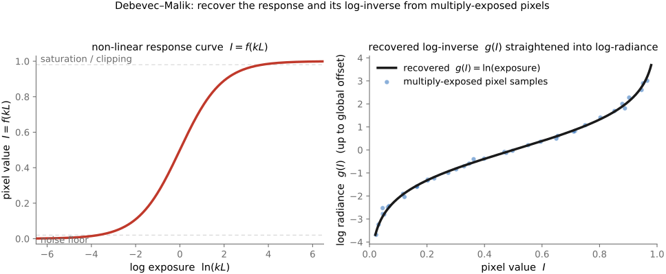
In the non-linear case, we need to recover the response curve. Real cameras (and film, and JPEG) apply a non-linear response $f$, such as a gamma, a tone curve, or a film characteristic, including the beauty curve that gives a camera its look (Why scene-linear looks dull, in Part 8, Basic image processing and ISP). Then $I_i = f(k_i L)$, and you must recover $f$ (equivalently its log-inverse $g = \ln f^{-1}$) before you can merge. The trick of Debevec and Malik (1997) is that a pixel imaged at several exposures gives several $(I_{p,i}, t_i)$ pairs that all constrain the same radiance $L_p$, and that over-determination pins down the curve. Here aperture and calibrated gain are fixed, so $k_i$ is the shutter time $t_i$ times a common scale, which is absorbed into $L_p$. Working in the log domain, each observation says

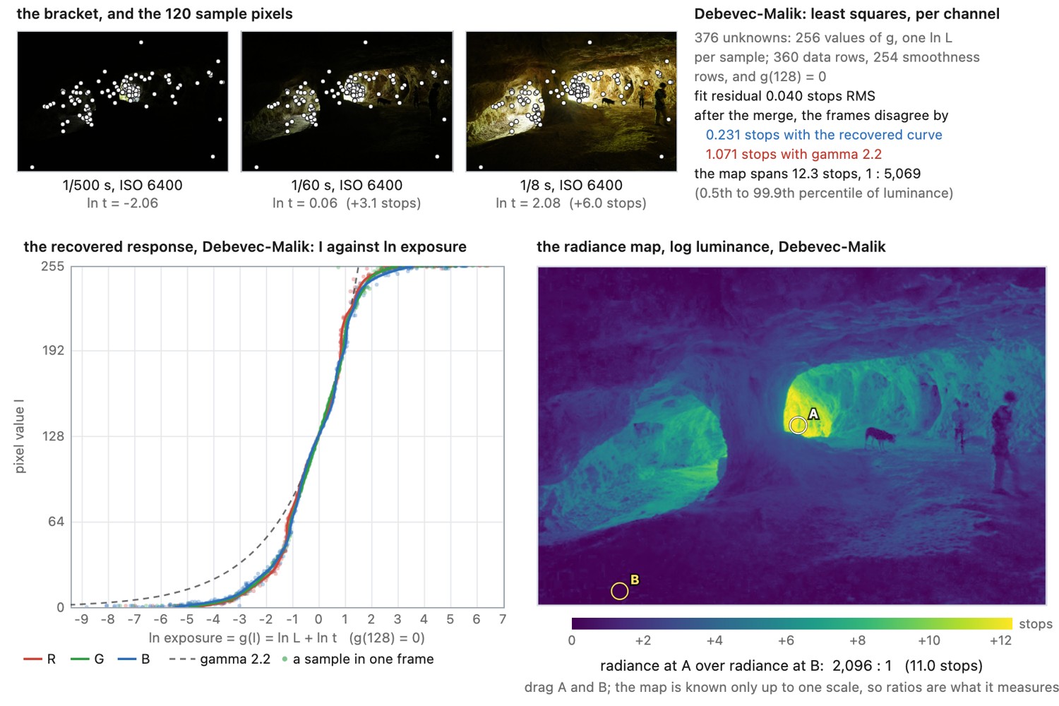
The unknowns are the curve $g(\cdot)$, one value per possible pixel level, say 256 of them, and one $\ln L_p$ per pixel. Stack one such equation per pixel per exposure and you have a linear least-squares system in $g$ and the $\ln L_p$'s, solved jointly, exactly the kind of inverse problem of Chapter 6.7, Image formation as a linear system. Two riders make it well-behaved: a smoothness penalty on $g''$ (a real response curve is smooth, not jagged), and the same reliability weight $w(I)$ we will use in the merge, down-weighting samples near the clip and near the noise floor. The recovered curve is fixed only up to one additive constant, again the global scale (Figure 17.2.2⛶ fullscreen).

With sample pixel $p$ and frame $i$, one explicit fit is

Here $\ell_p=\ln L_p$, the second sum runs over the possible pixel values $I$, $\Delta^2$ is a discrete second difference, and $I_{\rm mid}$ is a mid-range value whose $g$ is fixed. Fixing one curve value removes the additive-scale ambiguity. The written weights multiply residuals before squaring; using weights outside the square is a different convention. Smoothness alone does not enforce a monotone response. Check the recovered curve and held-out exposure residuals.

The system is small. Each $\ell_p$ appears only in its own sample's rows, so it can be eliminated exactly, leaving a symmetric 255 by 255 system for $g$ per channel that solves in milliseconds (Figure 17.2.1⛶ fullscreen). Run it on camera JPEGs and try three things. Set the weight to flat, and the clipped samples at 0 and 255 bend the ends of the curve. Lower $\lambda$ and the curve follows the noise; raise it and it can no longer turn at the toe. Merge with an assumed gamma of 2.2 instead of the recovered curve, and the frames of a bracket disagree about a pixel's radiance by about a stop, against a few tenths of a stop with the curve.

Mitsunaga and Nayar (1999) assume even less. They model the response as a low-order polynomial and recover it, together with the unknown exposure ratios, by radiometric self-calibration, so you need not even trust the EXIF exposure ratios. The spirit is identical: pixels seen at multiple exposures over-determine the curve, so fit a smooth response to them. (Mann & Picard 1995's "comparametric," or Wyckoff, work is the earlier multiple-exposure precursor to both.)

The figure runs their method as a second option on the same samples. Their model is the inverse response itself rather than its logarithm $g$: a polynomial of degree $D$, $f^{-1}(I) = \sum_{n=0}^{D} c_n I^n$, on pixel values normalized to $[0,1]$, with $f^{-1}(1) = 1$. Two steps alternate: with the exposure ratios $k_i/k_{i+1}$ of consecutive frames fixed, every pixel seen in both gives a linear equation $f^{-1}(I_{p,i}) = (k_i/k_{i+1})\, f^{-1}(I_{p,i+1})$ in the $c_n$, solved by least squares; with the curve fixed, each ratio is re-estimated as the average of $f^{-1}(I_{p,i})/f^{-1}(I_{p,i+1})$. Start the ratios a stop off EXIF, alternately up and down, and the iteration brings them back to within a few tenths of a stop. Start them all off the same way and it cannot. If $f^{-1}$ and the ratios $k_i/k_{i+1}$ explain the images, so do $(f^{-1})^{\gamma}$ and $(k_i/k_{i+1})^{\gamma}$ for any exponent $\gamma$, so the pictures fix the ratios only relative to one another, as Grossberg and Nayar showed Grossberg & Nayar 2003, and the polynomial model pins $\gamma$ only weakly. Run exactly as published on these JPEGs, the iteration drifts along that family, so the figure holds the bracket's total span in stops at its starting value, which removes that one direction and nothing else.

Joint fitting uses many observations while imposing a smooth response. It still requires sufficient exposure overlap and a suitable observation model. Debevec–Malik's conventional intensity weights are reliability heuristics, not automatically the inverse variances of log-transformed noise.

The log-domain estimate in Debevec–Malik is a weighted average of log exposures. Exponentiating it gives a geometric mean of radiance estimates, which differs from a linear-light arithmetic mean. Both can be useful under their respective error models; neither justifies averaging gamma-encoded values as radiance.

17.2.3 The pipeline end to end🔗⧉

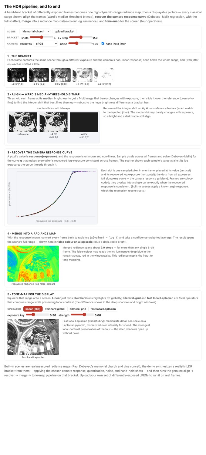
With calibration and combination both in hand, run the whole pipeline end to end, once, on one bracket: alignment, response recovery, merge, and (a preview of) tone mapping in a single interactive (Figure 17.2.3⛶ fullscreen).

17.2.4 From exposure to photometry🔗⧉

A shutter time, aperture and ISO setting can describe many scenes, including a lens cap left on. They establish a luminance only when connected to a known meter reading or an absolute camera calibration. The relative response calibration above also leaves an unknown scale.

For a specified reflected-light meter, at its recommended uncompensated exposure, the metering relation is

Here $L_v$ is the luminance represented by the meter reading, $S$ the arithmetic exposure index and $K$ its calibration constant in the stated unit convention. The expression describes the metered patch or weighting, not every pixel. If compensation $c_e$ adds stops at fixed ISO by increasing $t/N^2$, recovering the original meter-equivalent luminance requires multiplying the right-hand estimate by $2^{c_e}$. Manual settings unrelated to the meter support no such inference.

For an illustrative calibrated reading with $K=12.5$, f/2.8, 1/100 s, ISO 400 and zero compensation, $L_v=24.5$ cd/m². That is a meter-equivalent luminance under those assumptions. It is not an absolute estimate for an arbitrary photograph with those EXIF settings.

For a distant uniform patch, an idealized on-axis lens model relates that luminance to image-plane illuminance:

With transmission $\tau=0.9$, the example gives $H_v\approx0.0221$ lux·s. Off-axis pupil geometry, vignetting, flare and close-focus effects require more than this on-axis approximation. Calibrate black level, gain, linearity and spatial response for the actual camera and lens when absolute values matter Burggraaff et al. 2019.

A luminous exposure is weighted by human spectral sensitivity. It does not determine photon count without the spectrum. Given image-plane spectral radiant exposure $H_{e,\lambda}$, the expected detected electrons in a uniform photosite of area $A_p$ are

The factor $\lambda/(hc)$ converts energy to photons; quantum efficiency $\eta$ converts photons to expected electrons. Use wavelength units consistent with the spectral density. Replacing the spectrum by one average wavelength and one luminous efficacy is an additional approximation, not a consequence of the exposure settings.

To see the scale, complete the example under stated assumptions. Suppose the metered patch reflects broadband daylight whose luminous efficacy is about 300 lm/W over the visible band; this is an assumption about the spectrum, which the exposure settings do not supply. The radiant exposure is then $H_e \approx 0.0221/300 \approx 7.4\times10^{-5}$ J/m². Approximating every photon by its energy at 555 nm, $hc/\lambda \approx 3.6\times10^{-19}$ J, gives about $2\times10^{14}$ photons per square meter. A 4 µm photosite, $1.6\times10^{-11}$ m², receives about 3,300 photons, and with a flat quantum efficiency of 0.5 about 1,600 electrons, so shot noise alone limits its signal-to-noise ratio to about 40. A 1 µm phone photosite under the same exposure collects one sixteenth as much: about 100 electrons and a signal-to-noise ratio near 10, before read noise, and before the color filter passes only part of the spectrum to each photosite. That is the noise budget of Chapter 2.8, Noise, signal-to-noise ratio and dynamic range, and the reason merging frames matters on a phone.

Likewise, a nominal ISO label need not be the saturation-based ISO speed. A relation defining saturation-based speed cannot be applied to every manufacturer's recommended exposure index to infer sensor clipping or a fixed middle-gray headroom. Measure the relevant raw saturation and noise behavior.

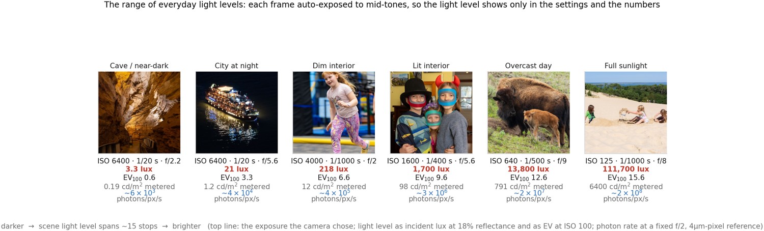
Across ordinary photographs the same chain spans a very wide range (Figure 17.2.4⛶ fullscreen). Six auto-exposed frames, from a near-dark cave to full sun, look about equally bright, yet their meter-equivalent luminances span more than four decades, about fifteen stops. The light level is invisible in the picture and shows only in the numbers: at the figure's reference lens and pixel, the near-dark end delivers a few thousand photons per pixel per second and is limited by noise, while the sunlit end delivers hundreds of millions. The exposure controls exist to slide that photon budget onto the sensor's usable range.