31.4 Refocusing and synthetic aperture🔗⧉

A light field is a recording you have not yet developed. In Chapter 31.1, Light fields 101 we saw that a conventional camera throws away an integral: every sensor pixel sums the whole cone of rays that the aperture lets through, a linear projection (Chapter 6.7, Image formation as a linear system) and once that sum is taken the individual rays are gone. With them go any choice about focus, aperture, or viewpoint, all of which were fixed the instant the shutter closed: Chapter 5.8, Photographic representation and its limits that recording the rays lifts. The light field keeps the rays. It is the function $L(u,s)$ that records, for each ray, the radiance crossing the aperture at position $u$ and the image plane at position $s$ (the full 4-D field carries the second aperture axis $v$ and the second image axis $t$; the 2-D slice $L(u,s)$ is enough to see every idea in this chapter). So the question for this chapter is the practical one: with all the rays in hand, what can you reconstruct?

The answer is that almost everything you would have decided at capture time becomes a choice about which rays you sum, and it is the same sum each time, only over a different set of rays. We will build up four reconstructions from the same operation: a normal photo, a stopped-down photo, a shifted viewpoint, and, most importantly, a refocused photo. Refocusing is shift-and-add, and sweeping it synthesizes a whole focal stack from a single exposure, which is exactly the dual of the real focal stack in Chapter 23.3, Focal stacks and depth of field extension. We close on the fast frequency-domain version (Fourier slicing), on reading both focus and depth straight off an epipolar slice, and on what happens when the aperture is not a lens but a camera array the size of a room: a synthetic aperture so large it sees through a fence.

31.4.1 Reconstructing a photo: it is all about which rays you sum🔗⧉

Start with the photo you would have gotten anyway. The hardware of Chapter 31.2, Light field cameras gives you, in effect, a grid of sub-aperture views: one small image of the scene as seen through each point $u$ of the aperture (in a plenoptic camera each microlens samples them; in a camera array each physical camera is one). A conventional photograph is the integral over the aperture: sum, at each scene point, all the rays that the open lens admits. In light-field terms that is simply: sum every sub-aperture view, pixel for pixel. Add up all the views and you are back to an ordinary, full-aperture photograph with its ordinary shallow depth of field. Nothing has been gained yet, but notice what we just did. We chose to sum all the rays. Every other reconstruction is the same sum over a different set.

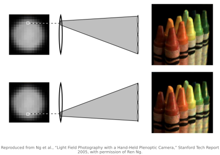
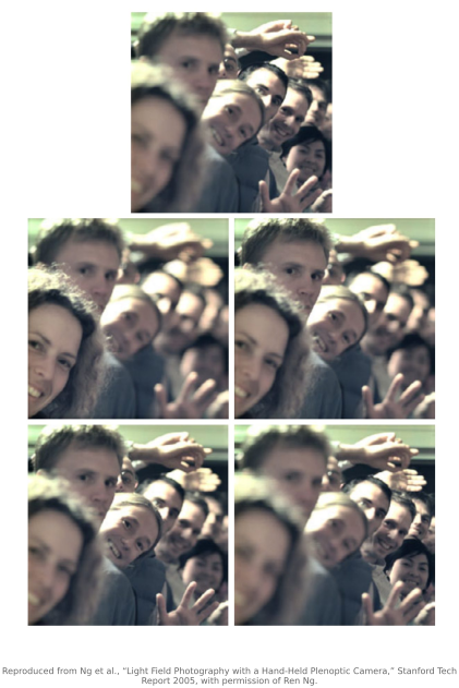
Digital stop-down. A smaller aperture admits only the rays near the center of the lens. So to stop the lens down digitally, sum the complete sub-aperture images associated with central pupil positions: discard the off-axis views, keep the ones near $u=0$. Fewer rays means less light, exactly as a real small aperture would, but it also means a deeper depth of field: the narrow bundle of central rays focuses to a tighter blur disc for off-plane points, just as the optics chapter said a small aperture would. You can dial the effective $f$-number after the fact, trading light for depth of field, by choosing how wide a patch of the aperture you integrate.

Viewpoint shift. Now go the other way: instead of summing many views, take just one ray per scene point, a single sub-aperture view at one fixed $u$. That is a pinhole image taken from one point of the lens. Pick a different $u$ and you get the scene from a slightly different vantage; the foreground slides against the background. That is parallax, and it is real 3-D information, but it is bounded: you can only move your eye as far as the physical aperture is wide, so the viewpoint shift is limited to the size of the lens (a camera array, with its wide baseline, buys you a far larger one). Drag the eye across the view grid and you see the scene rock back and forth, the same parallax that, in Chapter 31.1, Light fields 101, showed up as the slope of lines in the epipolar slice.

So: sum all the rays (normal photo), sum the center (stop down), take one ray (shift viewpoint). The remaining move is to sum the rays after shifting them. That is refocusing.

31.4.2 Digital refocusing is shift-and-add🔗⧉

A camera is focused on a plane when, for every scene point on that plane, all the aperture rays that left it land on the same sensor pixel. They converge, and the sum over the aperture is sharp. For a point off the focus plane the rays land spread out across several pixels, and the sum smears them into the blur disc. Refocusing means choosing a different plane to make converge. We cannot move the physical sensor after the fact, but we have all the rays, so we can ask where each ray would have landed on a sensor placed at a different distance (a virtual sensor) and sum there instead.

Work out where a ray lands on the virtual sensor and the whole operation collapses to a translation. Consider the view from aperture position $u_1$ versus the central view from $u_0$. A scene point at the new (virtual) focus depth projects, in the off-axis view, to a position offset from where it projects in the central view; by similar triangles, that offset is proportional to how far the aperture point sits off-center, $\lVert u_1 - u_0\rVert$, and to a constant $k$ set by how far the virtual sensor moved (Figure 31.4.2⛶ fullscreen). The constant of proportionality is the same for every scene point at that depth, which is what makes the correction a single rigid shift of the whole sub-aperture view rather than a per-pixel warp. To bring the new depth into focus, translate each view by the amount that cancels its parallax, then sum:

Read it back: for every aperture position $(u,v)$, slide that sub-aperture view by $(k u, k v)$ so that the chosen depth lines up, and add all the shifted views together. The weights $a(u,v)$ select and weight aperture samples; the denominator normalizes brightness for comparing apertures. Omit that normalization, and include calibrated radiometric weights, when computing collected irradiance. The simple shift form assumes rectified views with a fixed output scale. This is shift-and-add:

for every aperture location $(u,v)$: translate the sub-aperture image by $(ku, kv)$; add it into the accumulator. (We ignore the small field-of-view rescaling that the virtual sensor introduces.)

The parameter $k$ is the focus knob. At $k=0$ no view is shifted and you get the ordinary full-aperture photo focused at the native plane. As you change $k$, the shift you apply cancels the disparity of exactly one depth, and that depth comes into focus, its rays now stacking on top of each other, while every other depth, shifted by the wrong amount, blurs. Set $k$ and you have chosen, after the shutter, which slab of the scene is sharp. Note the family resemblance to the focal-stack merge of Chapter 23.3, Focal stacks and depth of field extension: there the in-focus slab was selected per pixel from captured frames; here it is synthesized by choosing one shift for the whole frame.

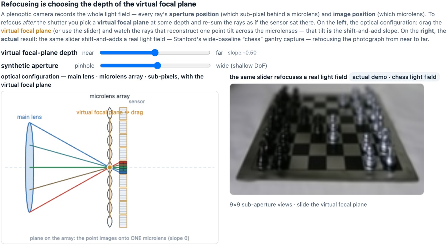
31.4.3 A focal stack from one capture, and an all-in-focus image🔗⧉

The shift $k$ is continuous, so nothing stops us from sweeping it. Sweep $k$ from front to back and you generate a whole focal stack, for example front-focused, mid-focused, and back-focused images, every frame computed from the one light field you captured (Figure 31.4.3⛶ fullscreen). This creates a computational counterpart of Chapter 23.3, Focal stacks and depth of field extension, with different sampling and noise limits. That chapter built a real focal stack by physically refocusing the lens between exposures, capturing $N$ frames; here we capture once and manufacture the same $N$ frames by shift-and-add. The focal stack defers focus by capturing frames; the light field defers it by capturing rays. Both are the same L13.1show move on the focus axis.

And once you have a focal stack, captured or synthesized, the rest of the machinery carries straight over. Feed the synthesized stack into the focus-stacking merge: measure local high-frequency energy per frame, take the sharpest at each pixel, and (in its principled form) cut and Poisson-blend along coherent seams. The high-exponent per-pixel sharpest selection, the photomontage of Chapter 23.3, Focal stacks and depth of field extension, collapses the whole stack into one all-in-focus image, with extended depth of field from a single exposure, limited by the captured spatial/angular bandwidth and the reliability of the focus measure. As a bonus, the per-pixel winning slope, which value of $k$ made each pixel sharpest, is a coarse depth map: the same shape-from-focus read-out, now obtained without ever moving the lens. One shutter press yields a refocusable stack, an all-in-focus image, and a depth map (Figure 23.3.8⛶ fullscreen).

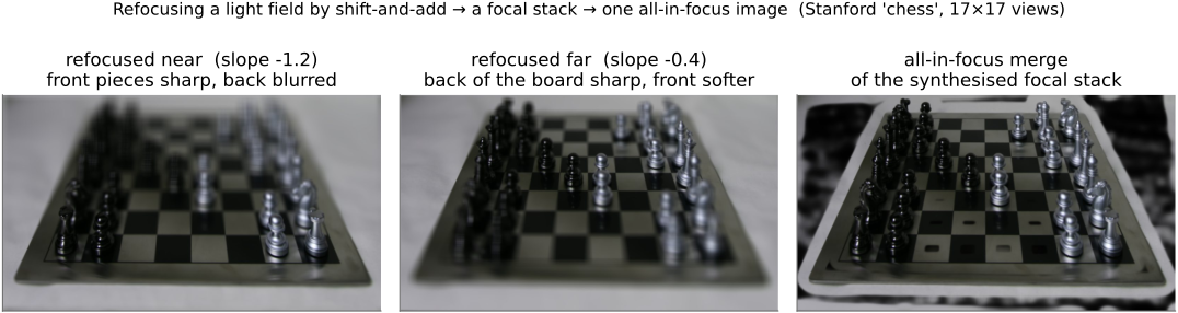
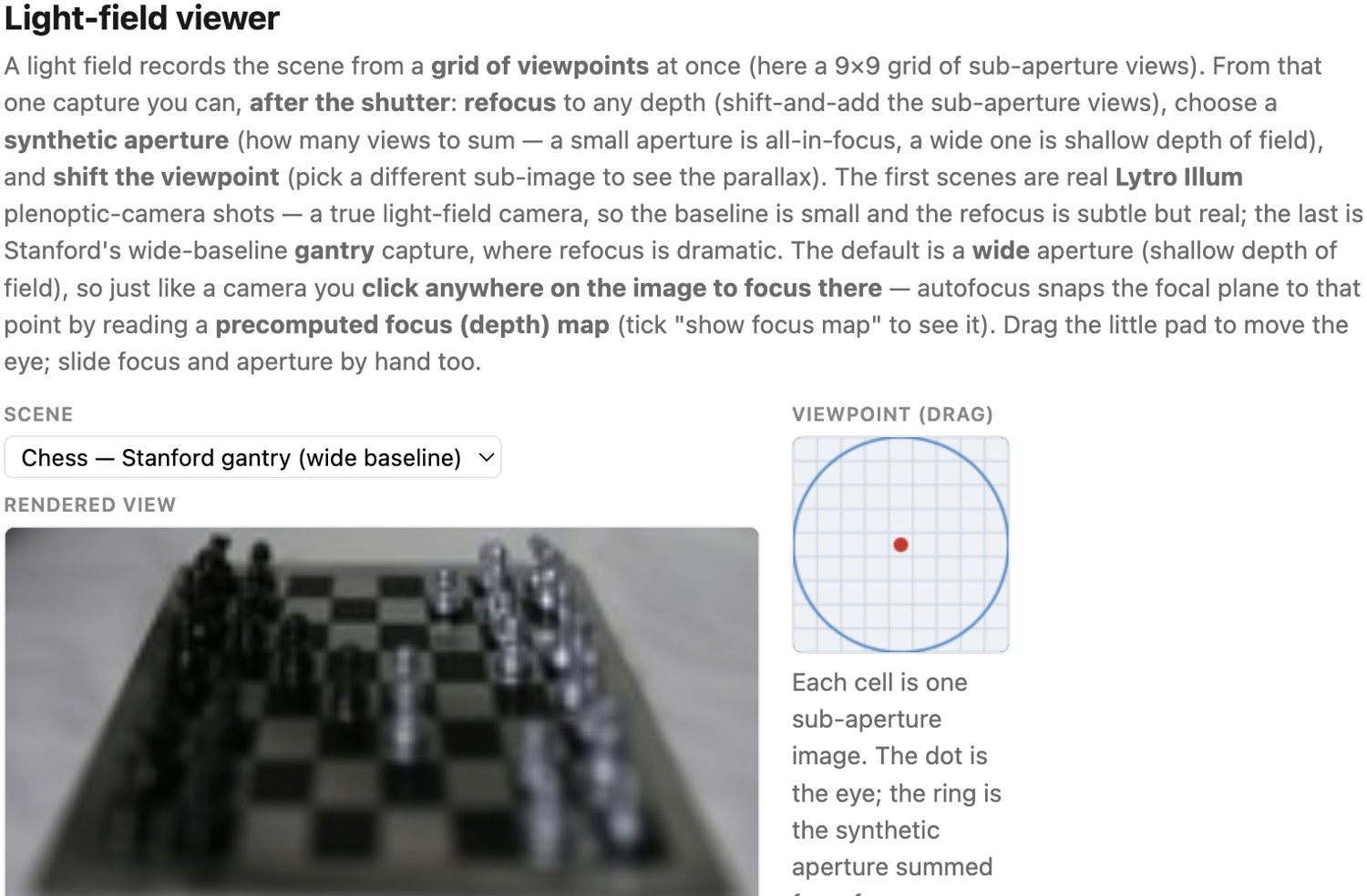
A plenoptic camera hands you, after the shutter, an image with the light-gathering and shallow depth of field of the full aperture, because you sum every sub-aperture view and keep all the photons, but with the freedom to place the focal plane anywhere within the depth of field of a single sub-aperture, whose effective pupil diameter is roughly the full aperture diameter divided by $n_a$, the number of angular samples across the pupil. Increasing $n_a$ can extend usable refocusing while reducing the simplest per-view spatial sample count for a fixed sensor. Here $n_a$ is a sample count; $k$ remains the refocus shear. This is the spatial↔angular trade once more. Two reconstructions sit on top, and they differ in kind: refocusing is linear: shift-and-add is a plain weighted sum of recorded rays, so it is cheap, stable, and well behaved; all-in-focus is non-linear: it is a per-pixel pick the sharpest frame selection (the focus-stacking merge of Chapter 23.3, Focal stacks and depth of field extension), data-dependent and therefore more fragile.

Noise accounting must compare the same output area and exposure. If a reconstructed pixel sums $n_a^2$ independent detector samples with total expected signal $S$ electrons and read-noise variance $\sigma_r^2$ per sample, its shot-plus-read variance is $S+n_a^2\sigma_r^2$. Summing retains their collected photons, but does not erase repeated read noise, optical losses, or resampling correlations. A single angular view uses only part of the available light. Focus selection is also noise-sensitive, though it may operate on refocused sums rather than on individual sub-aperture views. The spatial/angular budget and the photon budget are related through the hardware; resolution is not itself a photon count.

31.4.4 Fourier-slice photography: the fast version🔗⧉

Shift-and-add is intuitive but, done directly, it is $O(n^4)$: for one $n\times n$ output you sum $n\times n$ angular samples at every output location, assuming $n$ samples on each of the four axes. Ng 2005 found a far cheaper route by moving to the frequency domain. A refocused photo (the integral over the aperture of a sheared light field) corresponds, in the Fourier domain, to a 2-D slice through the 4-D spectrum of the light field, with the slice's orientation set by the focus depth. Recall the parallel from the focal-stack discussion: refocusing is a shear of ray space, and integrating over the aperture is a projection; by the Fourier projection-slice theorem, a projection in space is a slice in frequency, and a shear in space is a shear of that slice's orientation. So you transform the light field to its 4-D spectrum once, and then each refocused image is just a different sheared 2-D slice plus an inverse 2-D transform, giving approximately $O(n^2 \log n)$ per refocused image after the one-time 4-D transform, whose cost is $O(n^4\log n)$ under this equal-axis-size convention. The whole continuum of focal planes becomes cheap to explore once the spectrum is in hand. This is Fourier-slice photography, and it is one route to fast refocusing when the transform cost and storage can be amortized; direct GPU shift-and-add is another.

31.4.5 Reading refocus and depth off an epipolar slice🔗⧉

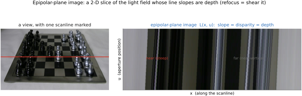
There is a single picture in which both depth and refocusing become geometrically obvious: the epipolar-plane image (EPI) from Chapter 31.1, Light fields 101, the 2-D slice of the light field at a fixed scene row, with image position $s$ on one axis and aperture position $u$ on the other. A scene point traces a line across this slice as you vary the aperture, and the line's slope is the point's disparity, hence its depth: near points slant one way, far points another, points on the focus plane run vertical. Now place the two operations of this chapter onto that picture. Depth is the slope you read off directly. Refocusing is a shear of the EPI: shift-and-add by $k$ skews the slice, and the depth whose lines the shear makes vertical, so they stack when you sum down the aperture axis, is the depth that comes into focus. Stop-down, viewpoint shift, refocus, depth: all four live as simple geometry in this one slice (Figure 31.4.5⛶ fullscreen).

31.4.6 Synthetic aperture: an aperture the size of a room🔗⧉

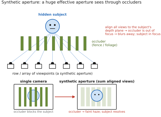
Everything so far used the rays inside one lens, so the synthetic aperture could be no wider than that lens. Replace the lens with a camera array, a grid of full cameras spread over a wide baseline, from Chapter 31.2, Light field cameras, and run the same shift-and-add, and the effective aperture becomes as large as the whole rig. The depth of field that results is extraordinarily shallow: a tiny slab in sharp focus, everything else dissolved into a strong blur. That sounds like a defect until you see what it buys.

Align the array (choose the shift $k$) to the plane of a subject hidden behind an occluder: foliage, a chain-link fence, a milling crowd. The subject, on its focus plane, has its rays brought into agreement across all the cameras, so their intensities reinforce one another and the subject becomes clearer. This is radiance averaging, not coherent optical interference. The occluder is at the wrong depth, so each camera sees it displaced differently; across the wide baseline a leaf that blocks one camera's view of the subject does not block the next camera's, and when you average all the views the occluder, never aligned, spreads into a veil whose strength depends on how many views it blocks. A point hidden from every camera remains unobserved; ordinary averaging does not remove all foreground attenuation or color contamination. The wide synthetic aperture has a depth of field so thin that the foreground is blurred almost out of existence while the plane behind it stays sharp. This is synthetic-aperture photography for seeing through occlusion, from Levoy et al. 2004 and Vaish et al. 2004, the dramatic extreme of the same shift-and-add we used to refocus a single lens, and a relative of the dynamically reparameterized light fields of Isaksen et al. 2000, which made exactly this choice of focal plane and aperture a control you steer after capture (Figure 31.4.6⛶ fullscreen).

A last connection. The light field is the common substrate under all the multiple-exposure ideas of Multiple exposure imaging: HDR varied exposure, panorama varied viewpoint, and focal stacking varied focus. A camera array can vary all of them at once across its many apertures. That generalization, from one synthetic aperture to many apertures fused for speed, dynamic range, and resolution, is the subject of the next chapter.