4.3 Encoding: linear, gamma or log⧉
Linear image values are proportional to the measured or represented light. An encoding maps them to stored numbers. The choice matters both for precision and for processing: adding encoded values generally does not add the corresponding light.
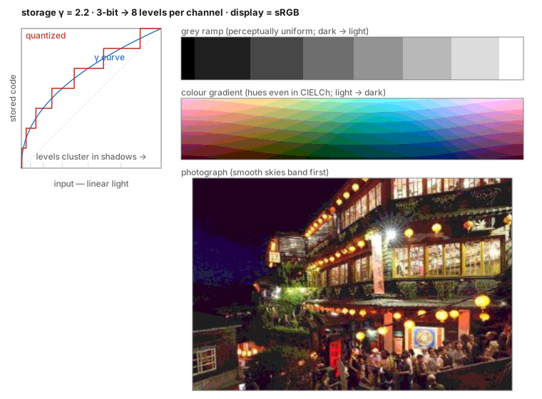
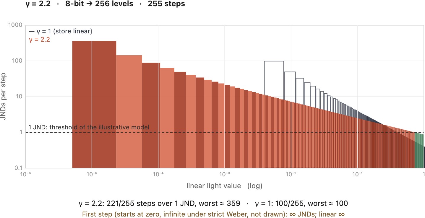
Uniform integer steps in linear light devote relatively few levels to dark regions. Human contrast sensitivity often depends more closely on relative than absolute differences, so a nonlinear encoding can use a limited bit budget more effectively Poynton 2012. This is an engineering approximation, not a universal law of brightness. Visibility also depends on the background, spatial structure, noise, and viewing conditions.
For example, a range of 100:1 divided into successive one-percent ratios needs about $\ln(100)/\ln(1.01)\approx463$ intervals. This motivates allocating codes by relative precision, but it does not prove that eight bits always suffice. Smooth gradients and subsequent editing can expose eight-bit quantization.
The name “gamma correction” encourages the wrong mental model. An encoding changes the numbers used to represent light; decoding reverses that change. There may also be a display nonlinearity to compensate and a deliberate contrast change to apply, but these are separate jobs even when all three involve power curves. Poynton's discussion emphasizes the continuing value of perceptual encoding after the original CRT motivation Poynton 2012. Removing an old display technology does not remove the need to allocate a finite code range according to visibility.
4.3.1 Gamma encoding⧉
For a simple power encoding on $[0,1]$,
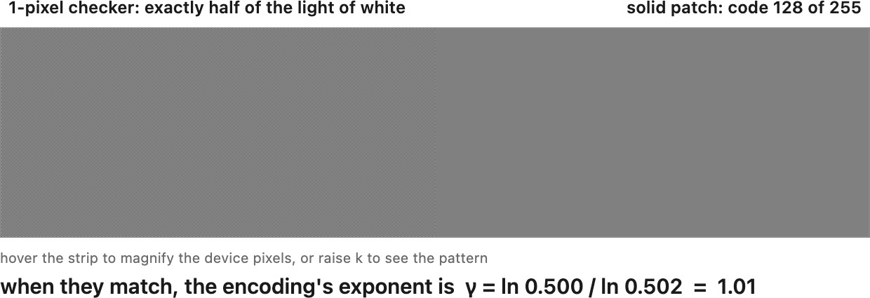
A value such as $\gamma=2.2$ moves code precision toward the shadows. It does not make all steps perceptually equal, and it is not the exact sRGB curve. I prefer “encode” and “decode” to the ambiguous “gamma correction”: name the direction and the actual transfer function.
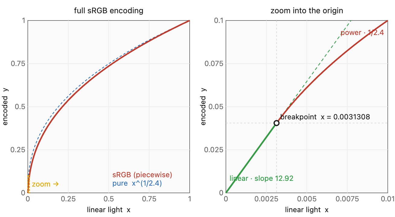
For sRGB, per channel,
and identically for $G$ and $B$. The prime does real work: $R'$ is what ships in the file, and $R$ is what you must convert to before any linear-light arithmetic. In code the pair is short, and worth keeping named so a caller can never confuse the two directions:
# sRGB OETF / EOTF, per channel, on values in [0, 1].
def srgb_encode(lin):        # RGB (linear) -> R'G'B' (gamma)
    return 12.92*lin if lin <= 0.0031308 else 1.055*lin**(1/2.4) - 0.055

def srgb_decode(enc):        # R'G'B' (gamma) -> RGB (linear)
    return enc/12.92 if enc <= 0.04045 else ((enc + 0.055)/1.055)**2.4
import numpy as np
def srgb_encode(lin):        # RGB (linear) -> R'G'B' (gamma); lin: array in [0,1]
    return np.where(lin <= 0.0031308, 12.92*lin, 1.055*np.power(lin, 1/2.4) - 0.055)

def srgb_decode(enc):        # R'G'B' (gamma) -> RGB (linear)
    return np.where(enc <= 0.04045, enc/12.92, np.power((enc + 0.055)/1.055, 2.4))
#include <cmath>
// sRGB OETF / EOTF, per channel, on values in [0, 1].
float srgb_encode(float lin) {   // RGB (linear) -> R'G'B' (gamma)
    return lin <= 0.0031308f ? 12.92f*lin
                             : 1.055f*std::pow(lin, 1.0f/2.4f) - 0.055f;
}

float srgb_decode(float enc) {   // R'G'B' (gamma) -> RGB (linear)
    return enc <= 0.04045f ? enc/12.92f
                           : std::pow((enc + 0.055f)/1.055f, 2.4f);
}
#include "Halide.h"
using namespace Halide;
// sRGB OETF / EOTF over a whole image (x, y, c), values in [0, 1].
Func srgb_encode(Func lin) {     // RGB (linear) -> R'G'B' (gamma)
    Var x, y, c; Func enc;
    Expr v = lin(x, y, c);
    enc(x, y, c) = select(v <= 0.0031308f, 12.92f*v,
                          1.055f*pow(v, 1.0f/2.4f) - 0.055f);
    return enc;
}

Func srgb_decode(Func enc) {     // R'G'B' (gamma) -> RGB (linear)
    Var x, y, c; Func lin;
    Expr v = enc(x, y, c);
    lin(x, y, c) = select(v <= 0.04045f, v/12.92f,
                          pow((v + 0.055f)/1.055f, 2.4f));
    return lin;
}
These snippets assume finite values in $[0,1]$. Working RGB may contain negatives or values above one, so a production implementation needs a documented extended-range convention; silently clipping before processing loses information. The rounded sRGB encoding junction differs by about $3\times10^{-8}$ in code value, not $10^{-4}$. Use the published constants consistently.
For a pure power curve at $N$ bits, the smallest positive decoded value is $(2^N-1)^{-\gamma}$. Its distance below white is $\gamma\log_2(2^N-1)$ stops. This describes the smallest positive code, not usable sensor dynamic range, and it does not describe sRGB’s linear toe. Eight-bit sRGB’s first positive code is about $1/(255\times12.92)$, roughly 11.7 stops below one. Neither count says how well intermediate tones are resolved or how far above noise a signal lies.
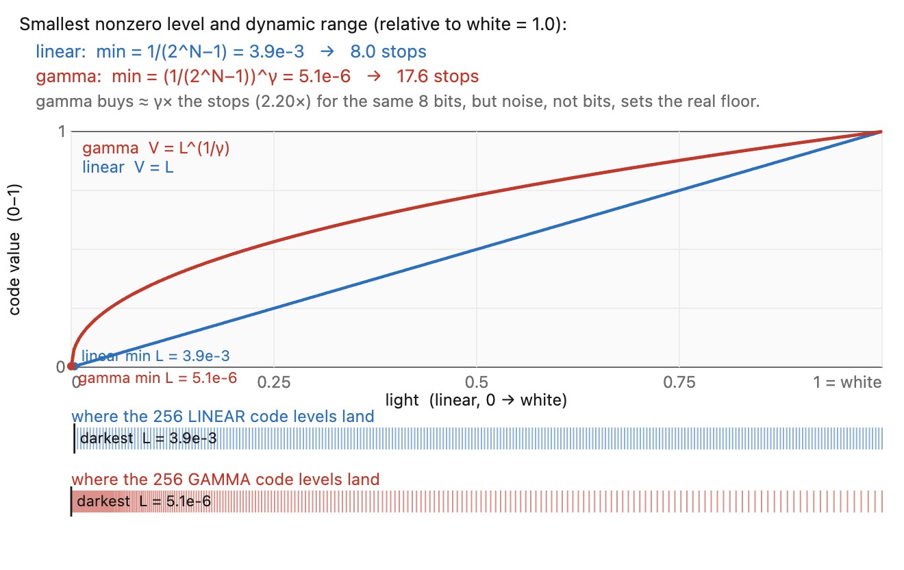
Historically, a CRT’s approximate power-law light output performed the decoding. Modern display systems reproduce a specified response through their electronics and calibration. Do not collapse all standards to “gamma 2.2”: Adobe RGB (1998) specifies a power near 2.2, ProPhoto/ROMM RGB uses 1.8 with a toe, and Rec. 709’s camera encoding is distinct from the BT.1886 reference display response, whose nominal exponent is 2.4. Apple's Macintosh used a system gamma of 1.8 for years, until Mac OS X 10.6 moved to 2.2 in 2009, which is one reason older untagged files can look too light or too dark on the other platform.
Film gamma is another quantity: the slope $\Delta D/\Delta\log_{10}H$ of optical density against log exposure in the straight part of a characteristic curve. It describes film contrast. An end-to-end scene-to-display rendering can intentionally change contrast; its transfer need not be the identity even when every encoding stage is correctly inverted.
A typical sRGB image file contains encoded values. Decode them for linear-light calculations, then supply the representation expected by the output interface. A viewer expecting sRGB needs sRGB-encoded output; a linear rendering surface may encode automatically. Encoding twice is as wrong as omitting it. RAW, log, HDR, and floating-point files require their own declared interpretation.
The application, operating system, GPU, and display share the output conversion. An embedded profile helps define the input, but it does not guarantee every application will honor it. Test the complete path rather than inferring it from the file extension.
For Rec. 709/sRGB primaries, relative luminance is $Y=0.2126R+0.7152G+0.0722B$ on linear values. Rec. 709 luma uses those coefficients on its nonlinear components. A common Rec. 601-style luma used with JPEG is instead
The coefficients and the encoding are independent pieces of the definition. Rec. 709 coefficients are not reserved for linear light.
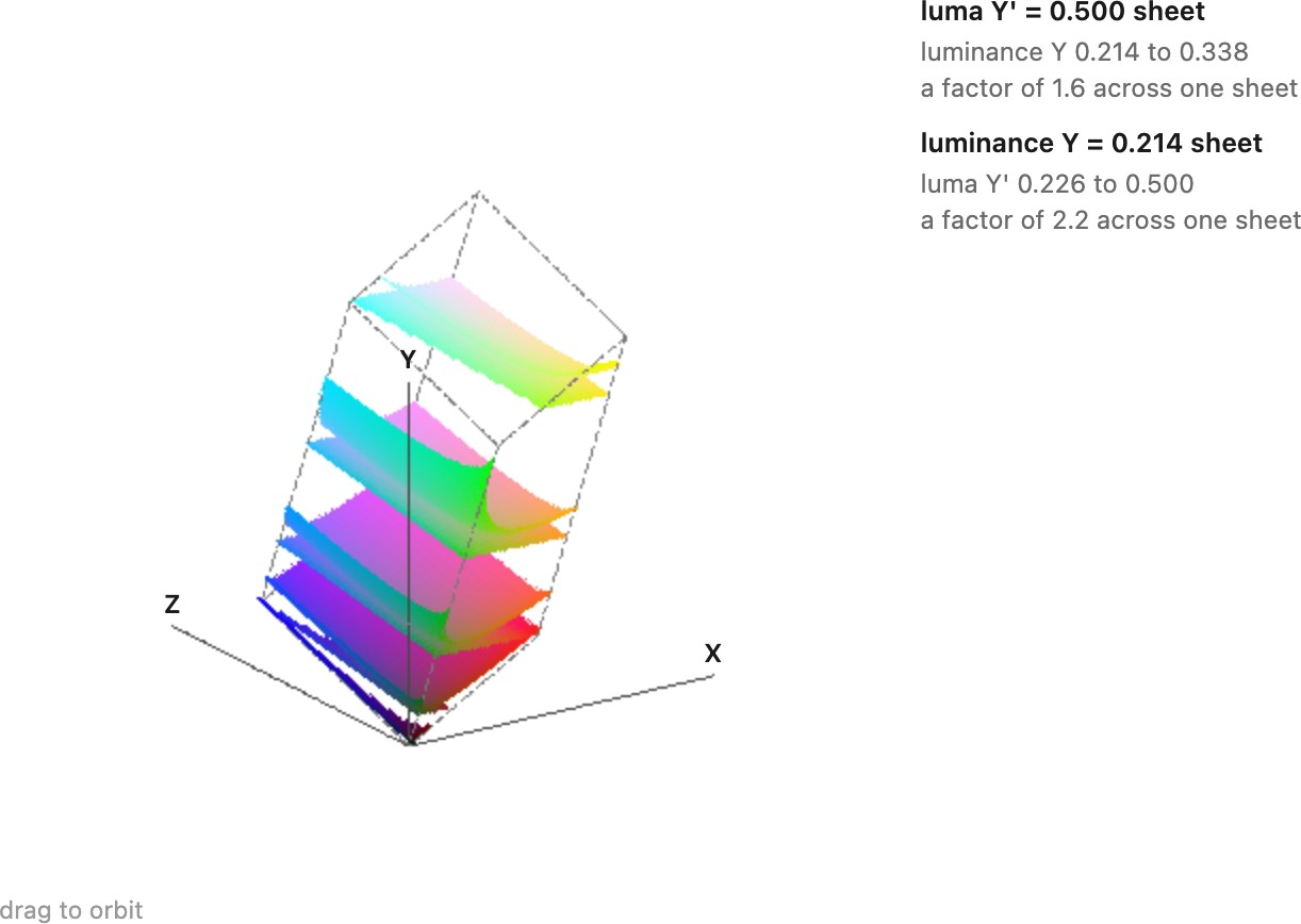
Luma is a weighted sum of specified nonlinear RGB components. Luminance is a photometric quantity obtained from linear values with the appropriate primaries and scale. Weighting and nonlinear encoding generally do not commute. Neither constant luma nor constant luminance guarantees equal perceived brightness across colors.
A simple level-counting calculation explains the attraction of nonlinear storage. Suppose, for this example, that adjacent displayed luminances should differ by at most one percent and that the brightest level is 100 times the darkest. Repeated multiplication by 1.01 needs about 463 intervals to span that range. At two percent, about 233 intervals suffice. These are illustrative constant-ratio thresholds, not a full visibility model: adaptation, spatial structure, and the display black level matter.
Compare that allocation with linear codes. Moving from code 1 to code 2 doubles the light; moving from 254 to 255 changes it by less than half a percent. The same absolute increment therefore buys very different relative precision. A compressive encoding allocates more codes to small linear-light values. Eight bits can still show banding, especially on smooth ramps, and a power law is not exactly the geometric spacing of a logarithm.
Transmission noise gives the encoding another job. Suppose approximately equal-sized errors are added to the encoded signal on its way to a receiver. Encoding has expanded the small linear-light values before that noise is added. Decoding then compresses an encoded error near black into a smaller absolute light error than the same encoded error near white. This is noise shaping, analogous to allocating quantization precision unevenly. It does not eliminate noise or guarantee constant visibility. The order is essential: noise added by the sensor before encoding has already affected the measurement, whereas channel noise added after encoding is subjected to the decoder's local slope.
The CRT joined this communication problem to a device constraint. Its approximate power response could perform the receiver's decoding as part of producing light. A modern system may distribute that job across application conversion, graphics hardware, display electronics, and calibration. The required input convention remains what matters to the programmer. Sending linear values to a path that interprets them as sRGB-encoded values applies the wrong relation between number and light, even if no individual component is broken.
A long pipeline also creates an ownership problem. The editor may convert a buffer that the operating system then converts again, or each may assume the other will perform a required conversion. The result is a double conversion or a missing one. An embedded profile is useful only if it still describes the numbers in the buffer and the next stage reads it correctly. A machine-checkable buffer type describing encoding, primaries, and image state would make these interface errors easier to catch. Keeping those labels explicit is the manual equivalent.
4.3.2 Gamma the contrast operator (gamma adjustment)⧉
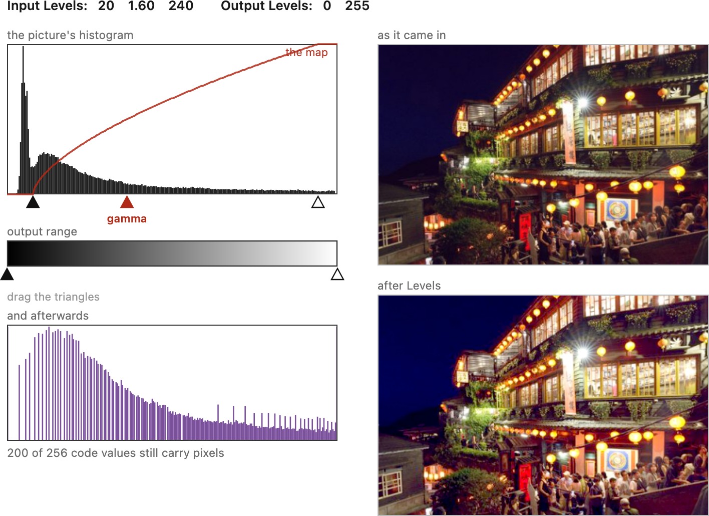
There is a second, entirely different thing called "gamma," and conflating it with the encoding is one of the classic color confusions. The gamma adjustment (the "gamma" slider in an editor) is a tone operator: it applies a power curve $V_\text{out} = V_\text{in}^{1/g}$ to the image to brighten or darken the midtones while pinning black and white, a midtone-contrast control. It has the same mathematical form as encoding gamma, a power law, which is exactly why the two get confused, but it is not the same thing: encoding gamma is an invertible change of representation before quantization; gamma adjustment deliberately changes the picture while leaving its encoding convention in place. A power edit can itself be inverted before clipping or quantization.
You meet it most famously as the middle slider in Photoshop's Levels dialog (Figure 4.3.7), the one between the black-point and white-point sliders. Levels maps input to output through a black point $b$, a white point $w$, an output range $[V_\text{lo}, V_\text{hi}]$, and a midtone gamma $g$:
with $w>b$ and $g>0$. Here $b, w$ set the input black and white points, $V_\text{lo}, V_\text{hi}$ the output range (usually $0$ and $1$), and $g$ (the middle slider, default $1$) is the midtone gamma: $g>1$ lifts the midtones, $g<1$ darkens them, both leaving the endpoints fixed. You can watch this exact control operate in the two ports of Photoshop 1.0 we ship, the original 1990 binary in an emulator and our line-by-line JavaScript re-implementation (Chapter 45.33, Photoshop 1.0, running, Chapter 45.34, Photoshop 1.0 ported to JavaScript), where the Levels code is a handful of lines and the gamma slider is literally an exponent. The lesson: when a tool says "gamma," ask which gamma, the invisible encoding you must respect, or the visible contrast knob you are turning on purpose.
4.3.3 System gamma: the end-to-end curve⧉
A third use of the word describes the whole chain rather than one stage. The end-to-end, or system, gamma is the slope, in log-log coordinates, of the curve from scene luminance to displayed luminance in the middle tones. If the display exactly undid the camera's encoding, it would be one, and the display would reproduce the scene's luminance ratios. Systems that look right use a system gamma above one, about 1.2 for a television in a dim room and up to 1.5 for a cinema in the dark, because a picture is seen under different conditions from the scene: a darker surround, a far lower absolute luminance, and flare in the room all make a faithful copy look flat. The system gamma is there to account for those viewing conditions; Chapter 18.1, Tone mapping and perception explains each effect.
The CRT made this convenient. Television cameras encoded light with an exponent of about 0.5 (the Rec. 709 camera curve is close to a square root), and a CRT's electron gun produces light roughly as the 2.4 power of its input. The display therefore did more than undo the encoding: the product of the two exponents, about 1.2, is the system gamma a dim living room needs. The physics of the tube happened to supply both the decoding and the perceptual tone mapping, which is one reason the BT.1886 reference display kept an exponent of 2.4 after CRTs disappeared.
4.3.4 Log encoding⧉
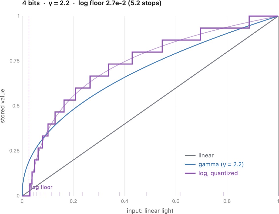
For positive light, logarithms turn exposure ratios into differences:
One stop is an increment of one. This is useful for exposure edits, relative contrast, and models of multiplicative illumination. Log values shift under a common gain; they are not themselves invariant. Differences between log values are invariant to that common gain.
Zero and negative values need an explicit policy. For a diagnostic log image, choose a positive floor $\epsilon$ in the same units as $L$, record which values were floored, and keep the reference scale fixed across images:
require epsilon > 0 and L_ref > 0
require all input values are finite
floored = (L < epsilon)
V = log2(max(L, epsilon) / L_ref)
# On unfloored samples only: L = L_ref * 2**V
A floor based on the smallest positive pixel varies with noise, crops, and frames, and fails on an all-black image unless separately handled. Flooring also destroys signed values. Camera log curves use specified toes and offsets; they are not this generic logarithm. Decode the named curve and range, such as LogC, S-Log3, or V-Log, before a scene-linear calculation. ACEScc and ACEScct are grading representations within ACES, alongside its linear representations.
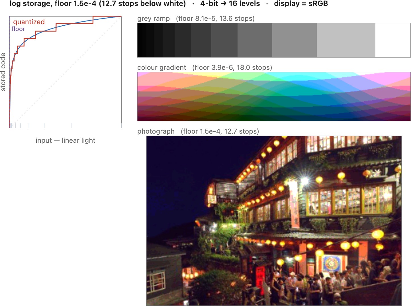
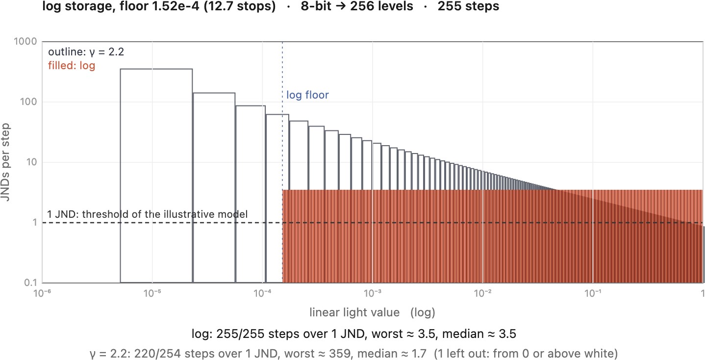
Homomorphic filtering and Retinex Land & McCann 1971 use logarithms to separate multiplicative factors under image-model assumptions. A high-pass log filter can suppress slowly varying illumination, but material color can vary slowly and shadows can have sharp boundaries. This is not a general recovery of reflectance.
Other uses include log-chromaticity methods, the Chong et al. space Chong et al. 2008, DIN99’s perceptual compression, and LogLuv image storage. Their objectives and definitions differ. Photographic density is $D=-\log_{10}T$ for transmittance $T$. Cineon represents printing density; its code increments are not scene-exposure stops without accounting for the film characteristic slope.
Use linear light for an operation that adds light. Use ratios or log differences when the model concerns multiplicative changes. Choose a perceptual encoding for storage precision or an edit defined in that representation. Log sharpening can be a legitimate contrast edit; it simply implements a different operator from sharpening linear light.
The following implementations expose the floor and reference value as explicit parameters. They implement the diagnostic mapping above, with a common contract: samples and parameters are finite, epsilon and reference are positive, and values below epsilon are replaced before the logarithm. The reference fixes the zero of the stop scale. Computing the difference of logarithms avoids overflowing the intermediate ratio for a very small reference.
import math

def to_log2(values, epsilon, reference=1.0):
    if not (math.isfinite(epsilon) and epsilon > 0 and
            math.isfinite(reference) and reference > 0):
        raise ValueError("epsilon and reference must be finite and positive")
    offset = math.log2(reference)
    result = []
    for value in values:
        if not math.isfinite(value):
            raise ValueError("samples must be finite")
        result.append(math.log2(max(value, epsilon)) - offset)
    return result
import numpy as np

def to_log2(values, epsilon, reference=1.0):
    if not (np.isfinite(epsilon) and epsilon > 0 and
            np.isfinite(reference) and reference > 0):
        raise ValueError("epsilon and reference must be finite and positive")
    values = np.asarray(values, dtype=np.float64)
    if not np.all(np.isfinite(values)):
        raise ValueError("samples must be finite")
    return np.log2(np.maximum(values, epsilon)) - np.log2(reference)
#include <algorithm>
#include <cmath>
#include <stdexcept>
#include <vector>

std::vector<double> to_log2(const std::vector<double>& values,
                           double epsilon, double reference = 1.0) {
    if (!(std::isfinite(epsilon) && epsilon > 0 &&
          std::isfinite(reference) && reference > 0))
        throw std::invalid_argument("epsilon and reference must be finite and positive");
    const double offset = std::log2(reference);
    std::vector<double> result;
    result.reserve(values.size());
    for (double value : values) {
        if (!std::isfinite(value))
            throw std::invalid_argument("samples must be finite");
        result.push_back(std::log2(std::max(value, epsilon)) - offset);
    }
    return result;
}
#include <Halide.h>
#include <cmath>
#include <stdexcept>

Halide::Func to_log2(Halide::Func input, float epsilon,
                    float reference = 1.0f) {
    if (!(std::isfinite(epsilon) && epsilon > 0 &&
          std::isfinite(reference) && reference > 0))
        throw std::invalid_argument("epsilon and reference must be finite and positive");
    // The caller checks sample finiteness before invoking this pipeline.
    Halide::Var x("x"), y("y"), c("c");
    Halide::Func output("log_encoded");
    Halide::Expr value = Halide::cast<float>(input(x,y,c));
    output(x,y,c) = Halide::log(Halide::max(value, epsilon)) / std::log(2.0f)
                    - std::log2(reference);
    return output;
}
For example, with reference=1 and epsilon=1/256, samples 1, 1/2, and 1/4 map to 0, -1, and -2 stops. A zero maps to -8. It can no longer be distinguished from a true 1/256 sample unless we retain the floor mask; the logarithm does not make discarded information recoverable.
The illumination–reflectance model also explains why logarithms recur in image processing. If an image is approximated by the product of an illumination field and a reflectance field, its logarithm is the sum of their logarithms. A spatial filter can then operate on the two contributions additively. Homomorphic filtering estimates a slowly varying component in log space, reduces that component, and exponentiates. Fine reflectance changes can retain their local contrast while broad brightness variation is compressed. Unfortunately, a broad material region can enter the low-frequency component, and a sharp shadow can enter the detail component. The decomposition is useful without being an exact physical separation.
Retinex Land & McCann 1971 connects comparisons across an image to color constancy. A ratio of two positive intensities becomes a difference of their logarithms. A common multiplicative gain cancels in that difference, which explains the appeal of relative comparisons. Spatially varying illumination does not cancel so simply. This connects log processing to Chapter 3.3, Adaptation and constancy and to the base/detail methods in Chapter 18.3, Two-scale and bilateral tone mapping.
Log recording and display encoding serve different stages. A named camera log curve can hold a broad range of scene values while making an exposure ratio correspond approximately to a code increment. That is convenient for grading. If those code values are sent directly to a display expecting sRGB, the picture usually looks flat because the intended rendering and display conversion have not happened. The flat appearance is not the goal of log capture. Decode the specified representation or use its defined rendering transform, then prepare the result for the target display.
Film density provides an older version of the same convenience. Multiplying transmittance changes optical density by an additive amount. Cineon's printing-density codes made that quantity available to digital grading. Converting a density increment into a scene-exposure increment also needs the film characteristic slope. For an illustrative straight-line slope of 0.6, one exposure stop changes density by about 0.6 times 0.301, or 0.181. If codes are spaced by 0.002 density units, that is about 90 code intervals per stop. Outside the straight part of the characteristic curve, the same calculation no longer applies. This accounts for the roughly constant-stop behavior without treating density itself as log scene exposure.
4.3.5 PQ, the perceptual quantizer⧉
PQ (SMPTE ST 2084, used by Rec. 2100) maps a normalized code $V$ to a nominal absolute display luminance $L_d$ up to 10,000 cd/m²:
where $m_1=2610/16384$, $m_2=2523/32$, $c_1=3424/4096$, $c_2=2413/128$, and $c_3=2392/128$, for $0\le V\le1$. For RGB, this transfer applies to the component signals; photometric luminance also depends on their combination.
PQ allocates precision using a contrast-sensitivity model. Ten-bit output does not guarantee invisible banding for every gradient, processing history, or viewing condition. A display may tone-map content outside its capabilities, so the specified luminance is a reference target rather than a promise about the actual emitted light. PQ can be paired with RGB and several component representations; it is not restricted to ICtCp.
4.3.6 HDR encoding⧉
HDR requires a sufficient numeric range and a defined interpretation of that range. The data type and transfer function do not, by themselves, determine whether an image is scene-referred or display-referred.
Floating-point scene-linear images are convenient for rendering, merging, and compositing. IEEE half precision has finite range: its positive normal values extend from $2^{-14}$ to 65504, about 30 stops. Subnormal values extend down to $2^{-24}$ with decreasing relative precision. OpenEXR supports half and other channel types. Values above one are ordinary working values; infinity is not valid unlimited image headroom. Radiance RGBE uses a shared exponent for three channels, reducing precision for small components beside a large one.
For HDR delivery, Rec. 2100 specifies PQ and HLG systems. HLG’s scene-light encoding combines square-root and logarithmic segments; its display system includes a viewing-dependent scene-to-display transform. It is relative, but it does not simply stretch every signal linearly to the panel peak. SDR compatibility is conditional on the playback path and does not mean every unconverted SDR display reproduces the intended picture.
Gain-map formats combine a base rendition with encoded gains and metadata for reconstruction at a different display headroom. The reconstruction applies the specified gains in the prescribed linear domain, with any offsets and weighting defined by the format. A gain map can vary in resolution and may have one or several channels. ISO 21496-1 standardizes this kind of representation. An older reader may show the base rendition while a supporting reader reconstructs HDR. Test both paths and preserve the metadata.
A scene-linear image still needs rendering for a particular display. Transfer encoding alone does not perform tone mapping or gamut mapping; see Chapter 18.2, Global tone mapping.
Floating point combines two useful properties. Its represented value is linear, so addition can still model light addition, while its exponent makes the spacing grow with magnitude. Within a normal exponent bin, the significand supplies the fine steps; moving to the next bin doubles both the scale and the step size. That is why a floating-point working image can cover a large range at approximately constant relative precision without applying a logarithm before every operation. A shared-exponent RGB format saves storage by choosing one scale for all channels, but a small component then has fewer useful steps beside a much larger one.
4.3.7 When to work on encoded values⧉
Choose the representation from the operator’s definition. Optical blur, radiometric exposure scaling, and physically based compositing require linear light. Quantization and compression often benefit from a perceptually motivated encoding. Tone curves can be deliberately defined on encoded values; that choice is part of the edit.
For denoising, use the noise model for the actual input domain. sRGB encoding is not a general variance-stabilizing transform. A square-root-like transform can approximately stabilize shot noise, but read noise, clipping, demosaicking, and later processing change that argument. The noise chapter derives the applicable models; do not import a uniform-noise denoiser merely because an image has been gamma-encoded.
4.3.8 Color and encoding in real pipelines⧉
A pipeline's choice of color coordinates determines what its operations mean. The same library can reconstruct radiance in one application and blend encoded samples in another. Follow the values through the implementation: where they become proportional to light, where an appearance transform changes them, and what the next stage assumes.
Consider an ordinary sRGB JPEG loaded into an array. Dividing its integer samples by 255 changes the numerical range; casting them to floating point changes the precision. Neither operation undoes the sRGB transfer function. A convolution will run on either array, and often produce a plausible picture. The programmer must supply the interpretation that makes its arithmetic meaningful.
The difference can occur within one library. OpenCV's detailed stitching sample loads images with imread, warps them, applies gain compensation, and feeds the result to a multiband blender. It does not decode a transfer curve along that path. With sRGB JPEG input, those operations therefore use encoded samples. Its HDR example, on the other hand, calibrates a response with createCalibrateDebevec, passes that response to createMergeDebevec, and tone maps the recovered HDR image. Response calibration and merging are separate calls. A convincing panorama and a radiance estimate impose different requirements on the same library.
A camera pipeline also has several reasons to change coordinates. Sensor corrections use calibrated measurements; later sharpening or chroma denoising may deliberately use encoded luma and chroma. Raw editors can provide perceptual controls between scene-linear stages. These choices are part of the rendering design. For a concrete example, darktable's documented scene-referred workflow keeps as much processing as possible in linear RGB and places tone compression late. Its display-referred workflow moves that boundary earlier. Even within the scene-referred workflow, a module can transform to another representation internally. “Scene-referred” describes the interpretation of an image, not a promise that every operation is linear.
RawTherapee's toolchain description makes the changes of coordinates visible: camera calibration and working RGB lead into operations that use Lab, followed by a conversion back to RGB for output. Its RGB and Lab comparison shows that similarly named saturation controls can produce different results because they operate on different coordinates. The working RGB profile alone does not specify the behavior of every photographic control.
The openISP reference implementation includes both early sensor processing and later luma/chroma filtering, edge enhancement, and hue/saturation controls. Such a design allocates different jobs to different domains. A luma denoiser after encoding does not have the same noise distribution as a denoiser on sensor measurements. These examples explain why a universal prescription to linearize an entire pipeline, or to keep the whole pipeline encoded, misses the purpose of individual stages. The detailed ISP discussion continues in Chapter 8.12, Recap ISP, non-destructive editing.
Panorama software provides another instructive comparison. Hugin's photometric optimizer models exposure, vignetting, white balance, and camera response. Its EMoR response model represents a curve with five coefficients. Matching overlapping scene points then involves correcting how the camera turned light into code values, rather than applying one gain to those code values and assuming that it represents exposure. The fitted model still depends on the images and the parameters chosen for optimization.
Enfuse has a different objective. It combines exposures using local measures of exposure, saturation, and contrast, based on the exposure-fusion method of Mertens, Kautz, and Van Reeth. It can produce a useful display image without first recovering a radiance map. Its success should therefore be judged as an appearance result. HDR reconstruction and exposure fusion can start from the same bracket but solve different problems; that difference explains why their treatment of camera response need not be the same.
Deblurring exposes the physical assumption especially clearly. A lens mixes incoming light before the camera encodes it. Encoding that mixture and blurring an already encoded image give different results, even without clipping. A reconstruction based on an optical convolution must account for this order. A learned model trained on stored RGB pairs can instead learn a mapping in that storage domain, but the training preprocessing then becomes part of its specification. Changing the test encoding changes the problem the model sees.
Graphics makes the conversion boundary explicit because light transport adds radiance. For example, the image implementation in Physically Based Rendering associates images with a color encoding and provides separate conversions to linear values and back. An encoded reflectance texture needs decoding before lighting. A normal map has vector components rather than encoded colors, even when both assets happen to arrive in the same file format.
A two-color mixture makes the error visible without a whole renderer. Equal amounts of linear sRGB red and green give $(0.5,0.5,0)$ in linear RGB, about $(0.735,0.735,0)$ after sRGB encoding. Averaging the encoded endpoints instead gives $(0.5,0.5,0)$ in code values, only about $(0.214,0.214,0)$ in linear light. In this symmetric example the chromaticity is unchanged but luminance is much lower. For general endpoint colors, the channel ratios can change too. A perceptual palette gradient can deliberately follow another path; a simulation of two mixed lights has this specific linear answer. The cross-fade figures in Chapter 4.9, Color TLDR compare these paths on patches and photographs.
4.3.9 What gamma buys, and what it costs⧉
Nonlinear encoding redistributes precision. It can also reshape the effect of noise added after encoding, as in a transmission channel. It does not recover sensor information, guarantee uniform noise, or make a power law invariant to illumination. If $V=L^{1/\gamma}$, multiplying $L$ by $a$ multiplies $V$ by $a^{1/\gamma}$; only a logarithm converts that multiplication into an additive shift.
The processing cost is that arithmetic changes meaning. Averaging encoded black and white and then sRGB-decoding gives about 0.214 units of light; averaging their linear values gives 0.5. A log average gives a geometric mean, with a result near black that depends on the floor. These are different operators, not three interchangeable implementations.
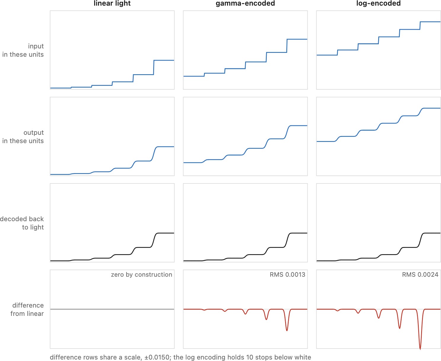
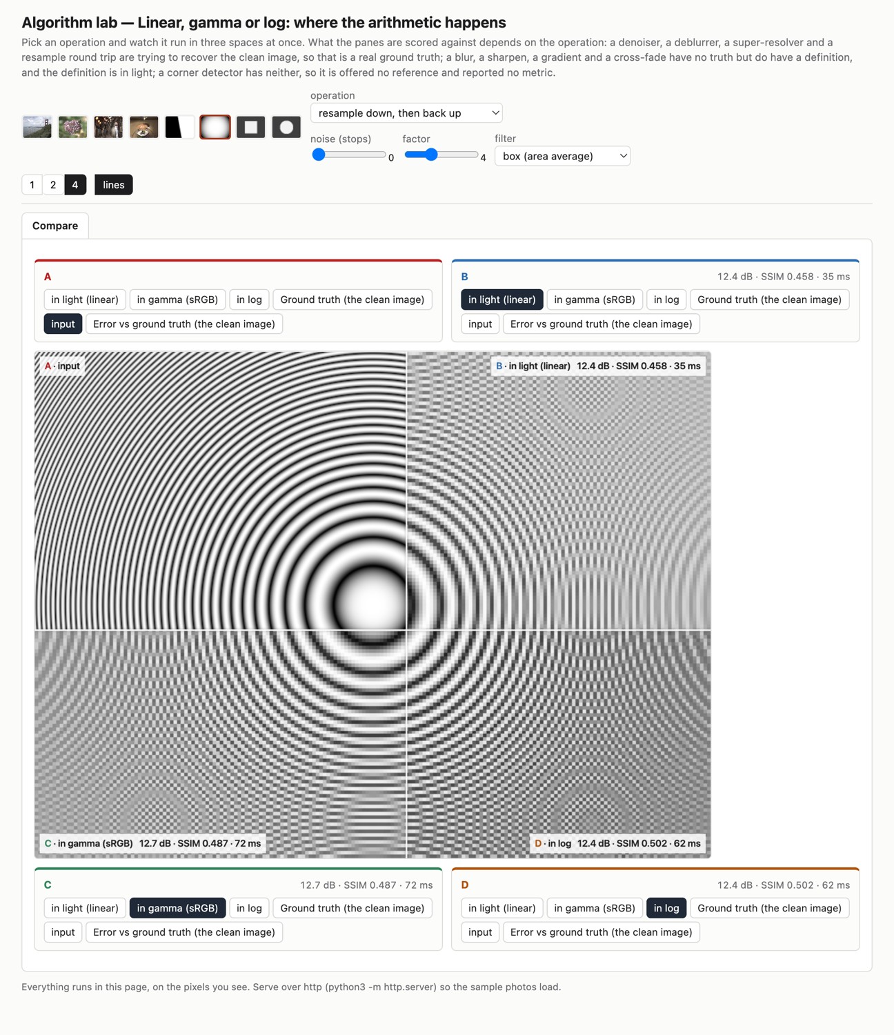
To average light, decode, combine linear values, and encode for the output interface. For nonnegative weights summing to one and a convex decoding curve, averaging encoded values produces no more light than averaging the decoded inputs. Kernels with negative weights need separate analysis. For alpha compositing, linearize color and use the correct premultiplied-alpha convention; alpha itself is not gamma-encoded color.
Recap: big lessons of this chapter
A typical sRGB image file contains encoded values. Decode them for linear-light calculations, then supply the representation expected by the output interface. A viewer expecting sRGB needs sRGB-encoded output; a linear rendering surface may encode automatically. Encoding twice is as wrong as omitting it. RAW, log, HDR, and floating-point files require their own declared interpretation.
Luma is a weighted sum of specified nonlinear RGB components. Luminance is a photometric quantity obtained from linear values with the appropriate primaries and scale. Weighting and nonlinear encoding generally do not commute. Neither constant luma nor constant luminance guarantees equal perceived brightness across colors.
Use linear light for an operation that adds light. Use ratios or log differences when the model concerns multiplicative changes. Choose a perceptual encoding for storage precision or an edit defined in that representation. Log sharpening can be a legitimate contrast edit; it simply implements a different operator from sharpening linear light.
To average light, decode, combine linear values, and encode for the output interface. For nonnegative weights summing to one and a convex decoding curve, averaging encoded values produces no more light than averaging the decoded inputs. Kernels with negative weights need separate analysis. For alpha compositing, linearize color and use the correct premultiplied-alpha convention; alpha itself is not gamma-encoded color.