4.2 White balance and white point⧉
White balance corrects an image for the scene illumination. A reference white defines a neutral stimulus for a color space or appearance calculation. A display also has a physical white, set by its calibration. These are related quantities, but they are not interchangeable.
For sRGB, equal linear RGB values have D65 chromaticity. ICC’s profile connection space uses a D50 reference. CIELAB accepts a specified reference white; D50 is an ICC convention, not a universal requirement of Lab. The ACES white is near D60. Specifying one of these whites does not itself apply an adaptation transform to an image.
I find the shared terminology unhelpful. A raw file may carry an as-shot white-balance estimate, the working RGB space has a reference white, and the output profile describes another device. Track which operation connects each pair. ACES makes input, working, and output transforms explicit, but it still has a defined working white and output viewing assumptions. It does not remove white adaptation from the rest of the pipeline. See the ACES white-point definition.
The light in the photographed scene and the light around the finished image play different roles. A tungsten-lit room may be shown on a monitor viewed in daylight; the viewer is no longer standing in the captured room. The rendering must decide how much of the scene's warm appearance to preserve under the new viewing conditions. Calling both sides “white” conceals that decision. The raw file's as-shot gains, the working space's reference white, and the calibrated display white are three pieces of information, not three instructions to neutralize the image independently.
This is why double adaptation is such an easy mistake. A conversion may already include the adjustment between its source and destination references. Adding another adjustment because the names D50 and D65 appear in the metadata applies the intended change twice. A pipeline with designated input and output transforms makes that responsibility easier to inspect. That is the useful architectural lesson from ACES; it does not depend on claiming that ACES has no working white or no later viewing adaptation.
4.2.1 Von Kries adaptation and white balance⧉
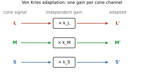
The von Kries model scales cone responses independently. Writing the three responses as $\mathbf r$, with source and destination white responses $\mathbf w_s,\mathbf w_d$, full adaptation takes the form
Division is componentwise, and the two whites must have a specified common normalization. Camera white balance similarly scales the camera’s linear channels, but these are sensor responses, not cone excitations. A diagonal transform in one basis is generally a full matrix in another. If $\mathbf c=M\mathbf r$, then
In general $MD\ne DM$. A common scalar exposure gain commutes with $M$; three unequal channel gains usually do not.
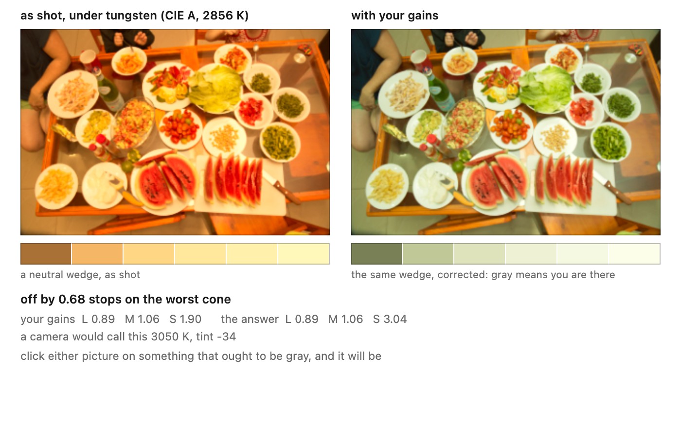
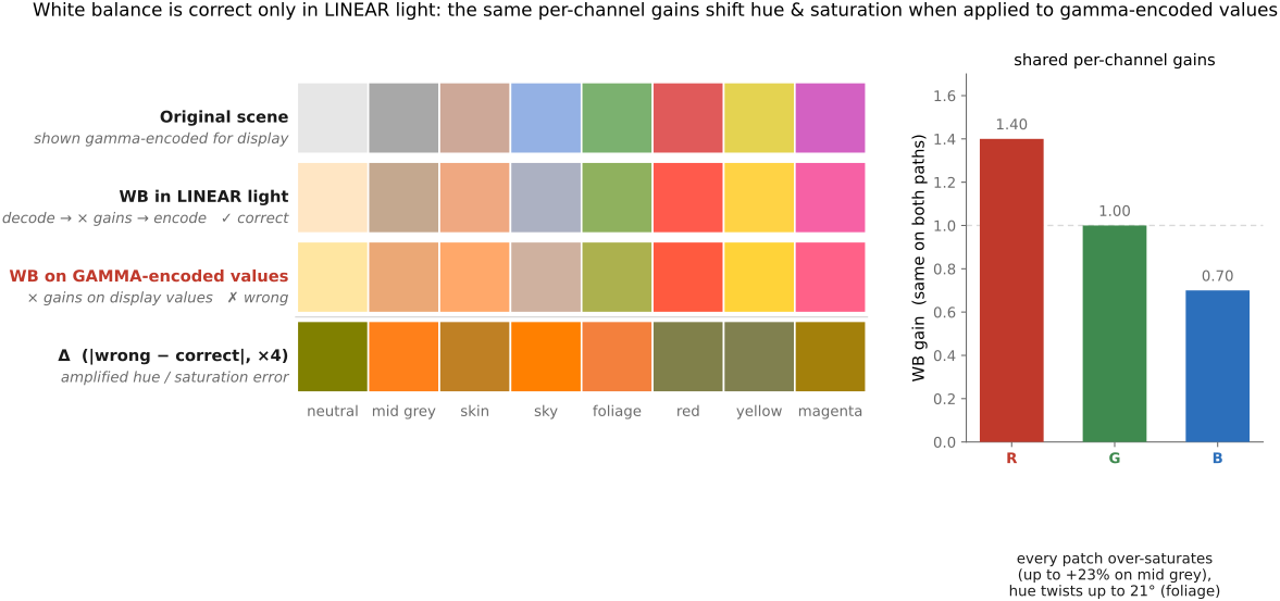
Apply physical channel gains to linear measurements, before clipping or tone rendering. For a pure power encoding $V=L^{1/\gamma}$, the gain $g$ on light corresponds to $g^{1/\gamma}$ on $V$. Applying the same gain to both representations gives different results. Real transfer functions can include offsets and piecewise segments, so decoding is the reliable way to implement a specified linear gain.
Temperature and tint are a convenient interface to illuminant chromaticity. Temperature follows the Planckian locus, obtained by integrating a blackbody spectrum against color-matching functions. Correlated color temperature (CCT) assigns a nearby locus temperature to a source that need not be a blackbody. It does not determine that source’s spectrum.
To construct the temperature axis, start with Planck's law for spectral radiant exitance,
Here $h$, $c$, and $k_B$ are Planck's constant, the speed of light, and Boltzmann's constant. Use compatible wavelength units, integrate this spectrum against the XYZ matching functions as in Chapter 4.1, Linear color reproduction and CIE XYZ, and normalize to chromaticity. A common multiplier cancels in that normalization. Repeating the calculation over temperatures traces the locus. Temperature supplies one coordinate along the curve; tint supplies a second direction away from it. This explains why two controls can describe a two-dimensional range of white chromaticities even though neither determines the full illuminant spectrum.
The standard signed distance $D_{uv}$ uses the CIE 1960 $uv$ diagram:
Near the locus, a model can specify $(u,v)_{\rm light}=(u,v)_{\rm Planck}(T)+D_{uv}\hat{\mathbf n}(T)$, with a chosen normal direction. Do not use CIE 1976 $v'$ in this formula; it is $3v/2$. Camera “tint” scales are application-specific and need not equal $D_{uv}$. Daylight models also differ from blackbody models. After removing common exposure scale, positive three-channel gains have two degrees of freedom; temperature and tint can parameterize a useful region of them. The mapping depends on the camera calibration.
4.2.2 How do you know the illuminant?⧉
A spectrally neutral, unclipped reference patch measures the illuminant through the camera sensitivities, up to a common scale. For its black-subtracted linear values $(R_n,G_n,B_n)$, gains
map the patch to $(g,g,g)$. Choosing $g=G_n$ leaves the green channel unchanged. Choosing the geometric mean makes the product of gains one; it does not generally preserve luminance. The raw developer’s subsequent camera transform must use the same normalization convention.
Average a patch rather than one noisy pixel. Reject clipped channels and values near the black level, where division is unstable. A wall that looks white may be colored, fluorescent, or lit differently from the subject.
Without a labeled neutral, automatic white balance estimates the illuminant using assumptions about scene statistics or learned scene content. Gray-world and white-patch methods illustrate those assumptions and their failures; the estimators are developed in Chapter 8.10, Auto-exposure and auto white balance.
4.2.3 White balance with mixed illuminant⧉
A face beside a tungsten lamp and a daylight window receives a spatially varying mixture of spectra. One global gain triplet cannot generally neutralize both sources. Local white balance estimates a gain field, but separating material color from illumination requires additional assumptions or user input.
The spectral model multiplies reflectance by the local sum of illuminant spectra before integration. A per-channel product of “material RGB” and “illuminant RGB” is only an approximation to that operation. Chapter 24.2, Mixed-lighting white balance develops methods that work with this ambiguity.
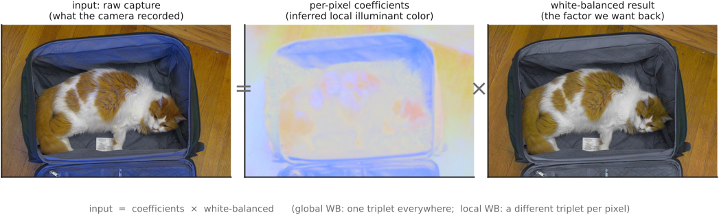
Consider a gray object between a warm lamp and a daylight window. Correcting the lamp-lit side with one set of gains can make the window-lit side too blue; correcting the window-lit side can leave the other side orange. A spatially varying correction is therefore a different estimation problem from choosing one white-balance triplet. In the approximate product model, each observed pixel combines three unknown material components and three unknown illumination components. Three measured channels cannot identify both triplets independently. A method must couple pixels through assumptions about surfaces, lighting, or user-specified neutrals. That coupling is what makes local correction possible, and also what can make it mistake a colored object for colored light (Figure 4.2.3).
4.2.4 White point in color space definitions⧉
An RGB space specifies primary chromaticities and a reference white. Let the columns of $P$ give primary XYZ directions with unit $Y$. Solve
Then $M_{\mathrm{RGB}\to\mathrm{XYZ}}(1,1,1)^T=\mathbf w$. This fixes the primary scales and luminance weights. It is a definition of coordinates, not a chromatic-adaptation model. Changing the reference white changes that definition; predicting how a stimulus should look under another adapting white requires an additional model.
Viewing adaptation may be partial and can involve both the image and its surround. A monitor’s brightest patch is not guaranteed to appear neutral regardless of its chromaticity. Color-management workflows specify reference viewing conditions so these assumptions can be shared.
The three roles should be named separately: a coordinate normalization, a physical display calibration target, and an assumption about the viewer's adaptation. They are often chosen to work together, but none logically forces the other two. The matrix equation above selects how much each primary contributes to the reference neutral. It does not establish what a viewer in an arbitrary room will perceive as white. My objection to the terminology is that a rendering assumption can become hard to see once it travels under the same “white point” label as the coordinate definition. Keep both in the specification rather than inferring viewing conditions from an RGB triplet.
4.2.5 Spectral sharpening within LMS space⧉
A chromatic-adaptation transform predicts corresponding colors across adapting conditions. A common linear Bradford implementation changes basis, scales the white responses, and changes back:
Here the whites and colors are XYZ. $M_A$ alone is the basis transform, not the complete white adaptation. For full adaptation with normalized whites, the complete transform maps $\mathbf w_s$ to $\mathbf w_d$. Source and destination white equal gives the identity, useful checks on an implementation.
rho_s = M_A @ source_white_XYZ
rho_d = M_A @ destination_white_XYZ
require every rho_s component is safely nonzero
adapted = solve(M_A, (rho_d / rho_s) * (M_A @ color_XYZ))
Bradford’s effective response functions are linear combinations of the XYZ matching functions Bradford chromatic-adaptation transform. They can have signed lobes. These are numerical coordinates, not new physiological cone measurements.
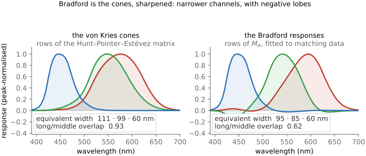
CAT16 supplies a different response basis in the CAM16 appearance model Li et al., CAM16 and CAT16 (2017):
The full appearance model includes adaptation degree and nonlinear response processing. Replacing the Bradford basis above with this matrix gives a full-adaptation transform, not all of CAM16. Use the transform required by the workflow: substituting CAT16 inside a profile conversion that specifies Bradford changes the conversion.
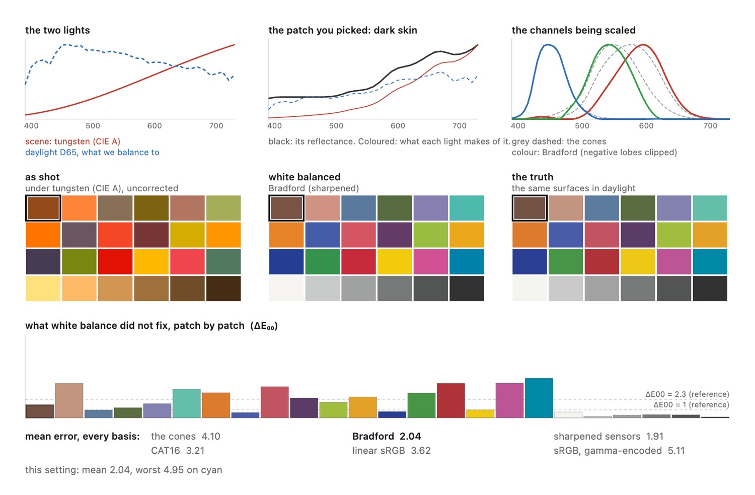
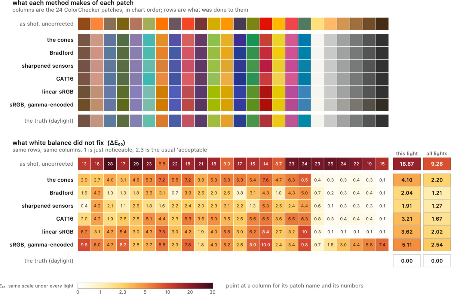
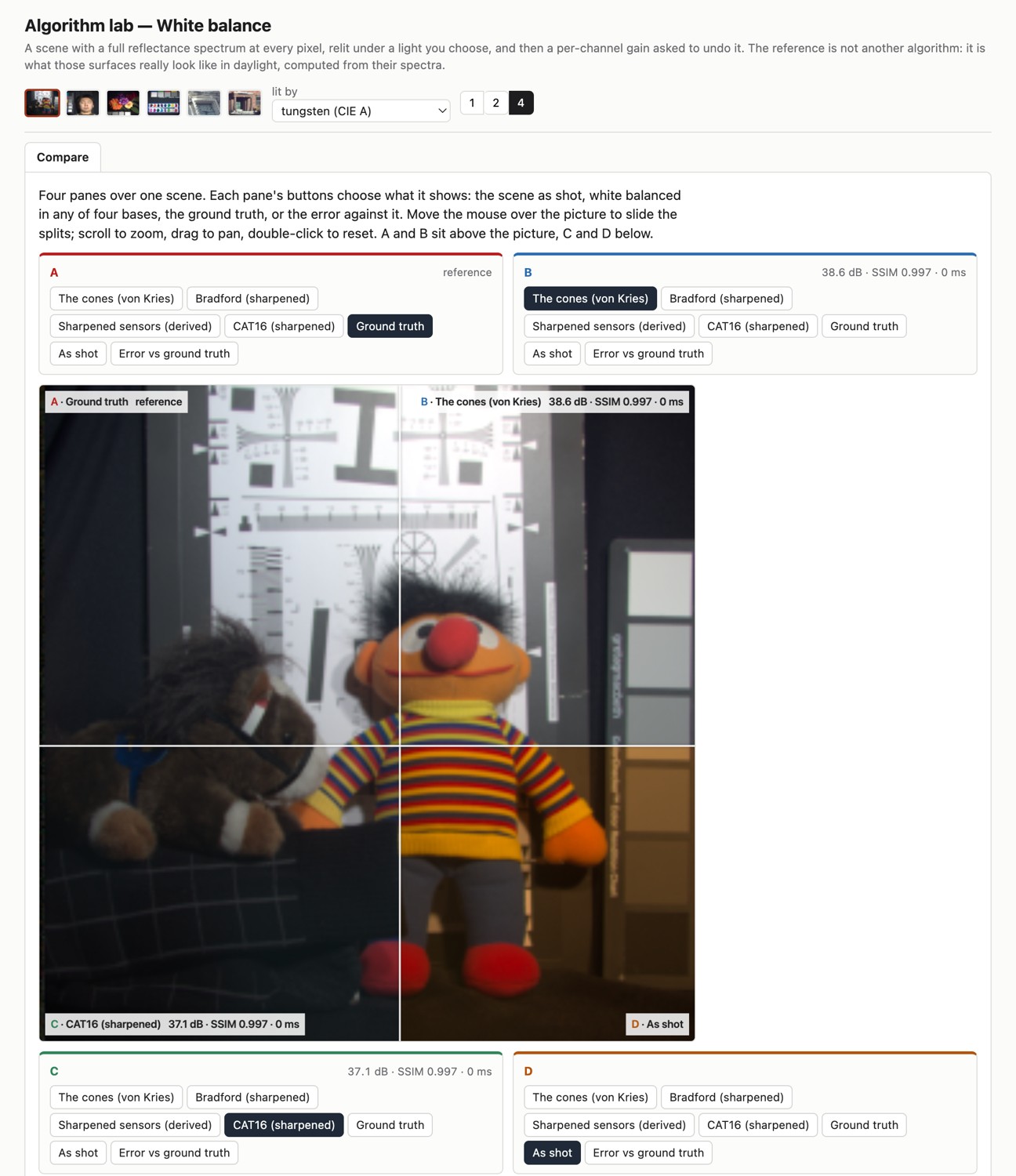
Corresponding-color experiments ask observers to match appearance under different conditions. Spectral relighting instead computes how the same reflectance responds to two illuminants. The figures below test the latter objective. Their rankings cannot establish which full appearance model best predicts people, and full adaptation is a valid limiting case rather than an inherently invalid test setting.
The architecture of the appearance model explains another difference between CAT02 and CAT16. CIECAM02 used one response space for chromatic adaptation and then changed to a Hunt–Pointer–Estévez response space for later processing. CAM16 instead performs the adaptation stages within one response space. Li and colleagues introduced this restructuring to address numerical and range problems while maintaining the model's fit to appearance data Li et al., CAM16 and CAT16 (2017). Thus the choice is about the surrounding model as well as the entries of an adaptation matrix. A comparison that substitutes only the three-by-three matrix does not test the whole architectural change.
Corresponding-color data and spectral relighting also answer different questions. In a corresponding-color experiment, a person chooses the patch that looks like a match under another adapting condition. That judgment depends on the surround, light level, and the observer. A spectral test instead measures or predicts what a fixed surface emits under the other illuminant. An appearance model can deliberately retain a cast when adaptation is incomplete, even though a physical relighting comparison rewards complete neutralization. Before reading a ranking of transforms, identify which target and which viewing assumptions generated the errors.
4.2.6 The limits of white balance, and CRI (color rendering index)⧉
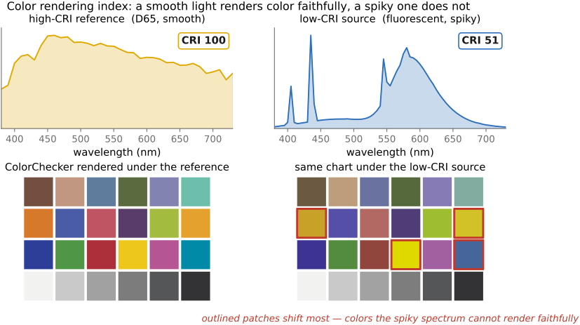
Two illuminants can have the same white chromaticity yet render colored objects differently. If a source delivers little or no energy in bands that distinguish two reflectances, three channel gains cannot recover the missing distinction. Even smooth illuminants need not be related by an exact diagonal correction.
The color rendering index (CRI) compares specified test colors with a reference source at a similar correlated color temperature. The commonly quoted general index $R_a$ averages eight test colors; it is not a complete assessment of saturated colors, preference, or camera fidelity. A high score does not specify the illuminant spectrum. Contemporary lighting specifications may also report more detailed fidelity and gamut measures. For photographic work, examine the actual source and the materials that matter, especially when mixing lights.
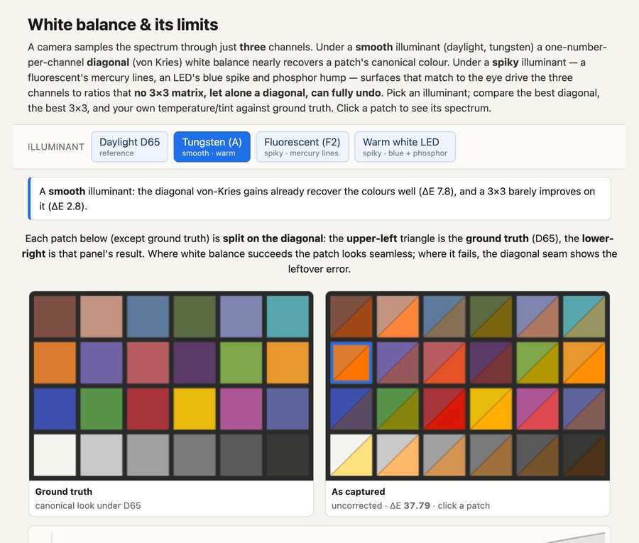
A matrix fitted on chart patches can reduce their residuals without accurately correcting other materials. Separate fitting and evaluation sets when testing a camera transform. Neither a low training error nor a neutral gray row establishes general spectral recovery.
4.2.7 Spectral sharpening with general spectra⧉
Spectral sharpening recombines measured channels to make their effective sensitivities more localized Finlayson, Drew & Funt, spectral sharpening (1994) Süsstrunk, Holm & Finlayson, chromatic adaptation sharpening (2000) Barnard, Ciurea & Funt, sensor sharpening for color constancy (2001). It can be applied to camera sensitivities as well as cone-based coordinates. A numerical three-by-three transform remains within the span of the original three sensitivities; it cannot synthesize arbitrary new spectral measurements.
For reflectance $r(\lambda)$, illumination $e(\lambda)$, and sensitivity $s_i(\lambda)$, a channel measures
A gain accurately models a change of illumination when the ratio of the two illuminant spectra is nearly constant across that channel’s effective support. Infinitely narrow sensitivities are one sufficient idealization; a common scalar change of illumination is another. Narrowing the effective support may help, but sharper is not universally better.
Numerical recombination also changes noise. For transform $H$ and input covariance $\Sigma$, the output covariance is
Large signed combinations can amplify noise and create channel correlations. A condition number alone does not give output noise variance. Nor does an invertible change of coordinates by itself destroy information; the practical costs arise in the operations, quantization, or clipping performed in those coordinates. Physically narrowing absorbing filters is different: it reduces detected photons under otherwise comparable conditions. The sensor noise model is developed in Chapter 2.8, Noise, signal-to-noise ratio and dynamic range.
For a simple example of the noise cost, subtract two channels that both respond strongly to the same broad spectral component. Their shared signal can nearly cancel while their independent read noise does not. If each channel has noise standard deviation one and the noises are independent, their difference has variance two and standard deviation about 1.41. Multiplying that small difference to make it a useful color coordinate multiplies the noise as well. Correlated channel errors change the calculation, which is why the covariance matrix matters. This is a numerical recombination of already captured photons. Placing a narrower absorbing filter in front of the sensor instead changes which photons are detected in the first place.
To see why localization helps, consider a channel that responds across both sides of a narrow peak in the illuminant. Two materials can put different proportions of their reflected energy under that peak while producing the same channel value under the original light. Under the new light they change by different factors. One gain cannot represent both changes. A more localized effective sensitivity samples a smaller range of those factors, which can make a diagonal approximation more accurate. Numerical sharpening seeks such useful combinations within the measurements already available; it cannot reveal spectral differences that all three original channels failed to distinguish.
4.2.8 Subjective white balance⧉
A neutralized gray card is useful for calibration, but it need not be the desired photograph. Candlelight and sunset illumination contribute to a scene’s appearance. A rendering may retain some warmth instead of fully discounting the light. Human adaptation itself is often incomplete.
Keep illuminant estimation, appearance prediction, and artistic preference separate. A dataset with measured neutral targets evaluates estimation. Corresponding-color experiments evaluate appearance matches. Expert retouches, such as MIT-Adobe FiveK Bychkovsky et al. 2011, provide examples of preferred rendering, though their edits include much more than white balance. Neither a person’s choice nor a manufacturer’s rendering is a unique physical ground truth.
Skin, sky, foliage, and the mood of the illumination can influence rendering decisions; see Chapter 4.5, Advanced color: opponents, perceptually-uniform, and preferred. Automatic systems can use scene content in both estimation and rendering, but a good result should not be interpreted as evidence that the illuminant was recovered exactly.
A candlelit dinner makes the distinction visible. A gray-card correction can provide a neutral reference, but applying it fully may remove the warm appearance the photographer wants to retain. Compare that neutral version with a partial correction: the latter leaves some cast while still separating skin from the orange illumination. Neither comparison requires treating one rendering as the true reflectance of every surface. The neutral reference is useful for calibration; the residual warmth is a rendering choice. A preferred white balance must therefore be evaluated with people and scenes, not only with a neutral-patch error.
This distinction changes how we diagnose a camera's output. Suppose a neutral target gives a reliable illuminant estimate, but the camera renders a tungsten-lit room warmer than a gray-card correction. The residual cast can be a deliberate choice about the photograph. Re-estimating the illuminant will not explain that choice; we need to inspect how the estimate is converted into rendering gains. Conversely, a camera can make an attractive image while estimating the illuminant poorly. A pleasing result by itself does not establish colorimetric accuracy.
A useful conceptual pipeline estimates the light first and chooses how much of its appearance to preserve second. It can fully neutralize a product photograph while leaving some warmth in a candlelit portrait. These choices need not be exposed as two separate controls, or even implemented as separate modules, but their objectives differ. The illuminant estimate can be checked against a reference target; the preferred warmth needs judgments about the rendered scene.
Scene recognition can enter both decisions. Recognizing a face may supply evidence about illumination, although skin reflectance varies and is not a gray card. It may also influence the desired rendering of skin after the light has been estimated. Sky and foliage raise similar distinctions between the measured color, the color a viewer remembers, and the color the photographer wants. A global white-balance gain changes the whole picture: independently adjusting skin, sky, and foliage requires additional selective color processing, as discussed in Chapter 4.5, Advanced color: opponents, perceptually-uniform, and preferred.
Manufacturer looks and user preferences add another choice. A rendering style can favor a warmer portrait or a cooler overall balance while starting from the same estimate of the light. Such choices are part of what photographers call a camera's color science, alongside its tone curves and selective color adjustments. They can differ between products and audiences; there is no single preferred white point that physics determines for every photograph.
The two kinds of training target therefore deserve separate treatment. An illuminant dataset records a physical reference and asks an estimator to recover it without seeing the chart. Expert-retouched photographs record choices about a finished image. The five retouchers in MIT-Adobe FiveK supply different renditions of the same inputs, which is useful precisely because preference need not have one answer. Their edits include exposure and tone as well as color, so using them to learn white balance requires distinguishing those operations. Scoring a preferred rendering solely by its distance from a neutral target would penalize some of the decisions it was designed to make.
An appearance model occupies yet another position. Its corresponding-color data asks what looks the same under different viewing conditions. That is an empirical model of human response, including incomplete adaptation. Preference asks what looks good. A mismatch to an appearance experiment calls for checking the viewing assumptions and model; a disagreement over the warmth of a photograph can remain after those are correct.
4.2.9 White balance datasets⧉
Public color-constancy datasets provide reference illuminants for training and evaluation. The common recipe runs the interactive figures above in reverse: photograph a real scene with a known neutral target in the frame (a gray card, a Macbeth ColorChecker, or a gray ball or cube), read the illuminant color off that target, then mask the target out so the algorithm has to recover the same illuminant from the scene alone. Accuracy is often reported as the angular error between the estimated and the true illuminant chromaticity, quoted as mean, median, and the worst 25%, since the hard scenes are the ones that matter. Two cautions run through all of them. The ground truth is only as trustworthy as the target and its placement: one card cannot describe mixed light. And the encoding of the released images matters enormously, black-level subtraction and whether the pixels are linear raw or already gamma-tagged shift the reported numbers, which is the well-documented source of the ColorChecker "reprocessing" discrepancies (Banić et al. on the ColorChecker dataset misuse).
Single-illuminant benchmarks, one global light per image, are the mainstay:
- Gehler-Shi ColorChecker, 568 raw images each with a ColorChecker: the canonical benchmark, and notorious because results from its two reprocessed versions (Gehler's and Shi-Funt's) are not comparable, owing to different black-level and linearization choices.
- NUS 8-camera (Cheng, Prasad and Brown), about 1,700 raw images of the same scenes shot on eight cameras: the standard test of cross-camera generalization.
- Cube+ and Cube++ (Banić et al.), Canon raw with a SpyderCube giving two neutral faces per shot: large, clean single-illuminant sets that anchored the ISPA color-constancy challenges.
- INTEL-TAU (Laakom et al.), 7,022 images across three cameras: one of the largest, built specifically to reduce camera and scene bias.
- SFU Gray Ball (Ciurea and Funt), 11,346 video frames each with a gray sphere in view: older and low-dynamic-range, but large and video-based, so it captures temporal illuminant changes.
Mixed and multi-illuminant datasets are the harder, more realistic frontier, exactly the regime where a single global gain cannot win:
- LSMI (Large-Scale Multi-Illuminant, Kim et al.), thousands of scenes lit by two or three sources with per-pixel illuminant ground truth.
- Multiple-illuminant / multiple light sources (Gijsenij, Lu and Gevers), the earlier laboratory-and-real set that defined the spatially-varying problem.
For post-capture correction, fixing the white balance of an already-rendered sRGB image rather than estimating a raw illuminant, the reference set is Rendered WB / When Color Constancy Goes Wrong (Afifi et al.): roughly 65,000 sRGB images rendered under many camera white-balance settings, for learning to re-neutralize a mis-balanced JPEG.
Finally, the spectral side of the problem needs images that carry the full per-pixel spectrum together with a known or controlled illuminant, so you can compute a reference illuminant chromaticity and predict the scene under another light within the measured spectral range, studying the metameric failures of the previous section directly rather than through one camera's fixed sensitivities:
- Foster et al. natural scenes, hyperspectral outdoor and indoor scenes, several captured with a small neutral (gray) reference in the frame so the illuminant spectrum can be read back and any other light substituted.
- Harvard (Chakrabarti and Zickler), 50 scenes under daylight plus 25 under artificial and mixed light, 31 bands, a natural test bed for known-versus-mixed illumination.
- CAVE multispectral (Columbia), 32 studio scenes at 31 bands shot under controlled illumination, with calibration details that must be checked before treating image values as reflectance.
- SFU spectral database (Barnard, Funt et al.), measured illuminant spectra alongside surface reflectances, the classic resource for synthesizing color-constancy scenes under an exactly known light.