13.5 Total variation and optimization-based denoising🔗⧉

A smooth sky contains noise fluctuations we would like to suppress, while its boundary against a building should remain sharp. Total variation makes this preference explicit by penalizing the sum of local gradient magnitudes. Unlike a squared-gradient penalty, it does not reward spreading a fixed contrast over many pixels.

For Gaussian noise of constant variance, the Rudin-Osher-Fatemi (ROF) model is

The data term penalizes departures from the observed image $y$; the TV term discourages variation. We have absorbed the likelihood's noise scale into $\lambda$, so its numerical value depends on the units of the image. This is the explicit-prior formulation of Chapter 7.1, Imaging as Bayesian inference with probabilistic priors (Rudin, Osher & Fatemi 1992 (TV)).

13.5.1 Why the penalty's shape decides the answer🔗⧉

Consider a one-dimensional edge of height $h>0$. A sharp jump contributes $h^2$ to a squared-difference penalty. Spreading the same change over $m$ equal increments contributes

The penalty alone therefore rewards a wider transition. An absolute-difference penalty instead assigns the sharp edge cost $h$ and the ramp cost $m(h/m)=h$. The data term can favor the sharp edge without having to overcome a larger regularization cost merely because the transition is concentrated (Figure 13.5.1⛶ fullscreen).

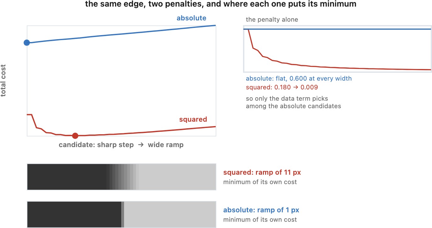
This comparison concerns the penalty, not the full minimizer. TV can still reduce edge contrast, displace boundaries, and remove small objects. It does not guarantee exact edge preservation.

The absolute value is also used in wavelet soft thresholding and in median estimation, but in different places. A median minimizes absolute data residuals; TV applies an absolute or Euclidean norm to spatial differences. Changing the residual loss changes robustness to outliers. Changing the gradient penalty changes the preferred image structure.

13.5.2 Isotropic, anisotropic, and the staircase🔗⧉

Let $Kx=(D_hx,D_vx)$ be horizontal and vertical forward differences on a unit-spaced pixel grid. We use zero outward differences at the image boundary. Isotropic discrete TV is

Anisotropic TV instead sums $|(D_hx)_p|+|(D_vx)_p|$. The Euclidean norm treats gradient directions more uniformly; the discrete grid still prevents exact rotation invariance. The anisotropic norm has a stronger preference for grid-aligned structures.

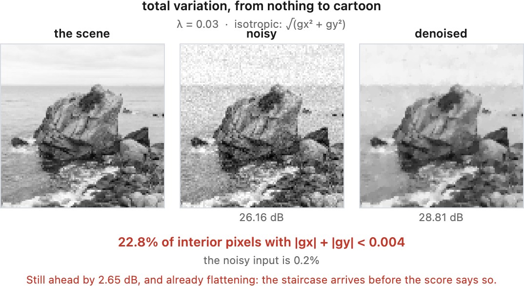
TV favors sparse gradients, so gradual shading can become flat plateaus separated by steps. The resulting staircasing is especially visible on skies and skin under strong regularization (Figure 13.5.2⛶ fullscreen). Total generalized variation introduces an auxiliary field and higher-order variation to allow gradual changes more readily (Bredies, Kunisch & Pock 2010 (TGV)). It is a different prior with its own weights, not just the same algorithm at the same numerical strength.

13.5.3 Solving it🔗⧉

The ROF objective is convex and has a unique minimizer because its data term is strictly convex. The gradient norm is not differentiable at zero. A primal-dual method handles this through a projection rather than replacing the norm by a smoothed approximation (Chambolle & Pock 2011 (primal-dual)).

Let $K^*$ be the exact discrete adjoint of $K$: $\langle Kx,p\rangle=\langle x,K^*p\rangle$. It is the negative divergence under the stated boundary convention. The following iteration solves the objective written above. The dual variable $p$ has two components per pixel and is projected onto a Euclidean ball of radius $\lambda$:

x = y
xbar = x
p = zero_gradient_field()
for iteration in 1..maximum_iterations:
    q = p + dual_step * K(xbar)
    p = q / max(1, vector_norm(q) / lambda)     # pointwise projection
    x_new = (x - primal_step * K_adjoint(p) + primal_step * y) / (1 + primal_step)
    xbar = 2*x_new - x
    x = x_new

Choose positive steps $\tau$ and $\eta$ with $\tau\eta\lVert K\rVert^2<1$. Unit-grid forward differences have $\lVert K\rVert^2\le8$, so $\tau=\eta=0.25$ is a conservative example. For $\lambda=0$, return $y$ directly. The update uses $-\tau K^*p$, or equivalently $+\tau\operatorname{div}p$; mixing these sign conventions solves the wrong iteration. Use a primal-dual gap or an appropriate convergence criterion when reporting an optimized result; a fixed iteration count is a computation budget.

Chambolle's dual algorithm provides another projection-based route (Chambolle 2004 (dual TV algorithm)). Split Bregman and the alternating direction method of multipliers (ADMM) Boyd et al. 2011 (ADMM) introduce $v=Kx$ (Goldstein & Osher 2009 (split Bregman)). With scaled dual variable $u$ and penalty $\rho>0$, the updates are

Here vector shrinkage is $\operatorname{shrink}_t(a)=\max(1-t/\lVert a\rVert_2,0)a$, with output zero at $a=0$. The first step solves a quadratic problem, the second shrinks gradient vectors, and the third updates their disagreement. Replacing this gradient shrinkage directly by an image denoiser would mix incompatible variables. Chapter 13.11, Denoising as a universal prior instead splits with an image copy so that its prior step acts on images.

13.5.4 Where it stands now🔗⧉

TV is a useful baseline when a preference for small total gradient magnitude fits the scene. It requires no training set, has an explicit objective, and supports convergence checks. Texture loss, contrast reduction, and staircasing limit it as a general photographic denoiser. A more accurate solver cannot remove an artifact preferred by the objective itself.

For a known blur or sampling operator $A$, replace the data term by $\tfrac12\lVert Ax-y\rVert^2$. The TV prior remains the same, while the data step changes. Non-Gaussian observations require a different likelihood. This separation of measurement model and image penalty is also useful in tomography and other reconstruction problems whose images and noise differ from ordinary photographs.