45.23 Reading a Lytro light field⧉
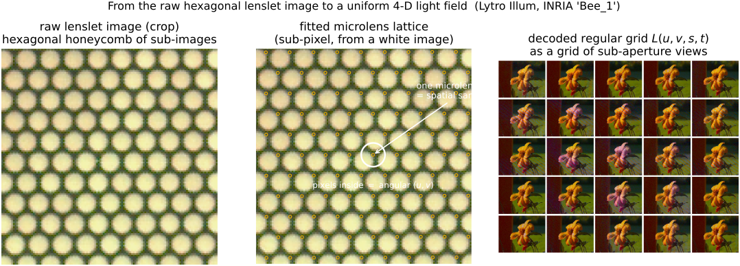
A Lytro .lfr is not a picture, and it is not yet a light field either. It is a single sensor frame, a lenslet image (a honeycomb of thousands of tiny circular sub-images, one behind each microlens; see Chapter 31.2, Light field cameras), plus a bundle of metadata describing the camera that made it. The 4-D light field $L(u,v,s,t)$ is in there, but sampled on a lattice that does not align with a rectangular pixel grid: the microlenses sit on a hexagonal grid, rotated by a fraction of a degree relative to the sensor rows, with a pitch of ~14 pixels that is not an integer and does not align with the Bayer mosaic underneath. "Decode it" hides two different jobs:
- The container job: get the bits out: parse the
.lfrwrapper, unpack the raw sensor frame, and read the metadata (the microlens geometry, the color tags, the black/white levels). This is container parsing, and a library does it for us. - The geometry job: put the rays on a uniform grid: locate every microlens center to sub-pixel accuracy, then resample each sub-image onto a regular $(u,v)$ angular block and each microlens onto a regular $(s,t)$ spatial lattice, converting the rotated hex sampling into the rectangular 4-D array $L(u,v,s,t)$ that every downstream algorithm wants. This is the hard part, and it is what this appendix is really about.
The microlens lattice is the whole problem. Estimate it to sub-pixel accuracy (ideally from a flat white image, not from the metadata alone) before you resample. The uniform grid you are building is an interpolation of the real lenslet centers; if your lattice is off by even a fraction of a pixel, or you forget that the rows are hexagonally staggered, the regular grid beats against the true one and you get banding and cross-talk that no later step removes. Get the geometry right first; everything else (color, exposure) is a normal-imaging problem layered on top.
45.23.1 The container: the LFP/LFR format⧉
A .lfr (and the older .lfp) is a simple chunked container. It opens with an 8-byte magic header (\x89LFP\r\n\x1a\n), then a sequence of length-prefixed sections each tagged by a magic word (LFM for a metadata chunk in UTF-8 JSON, LFC for a component of binary data) and identified by an embedded sha1-… string. One JSON metadata chunk is the table of contents: it names, by sha1, the chunks holding the raw image, the per-frame metadata, and a JPEG thumbnail. The raw sensor data itself is 10-bit, packed four pixels into five bytes (the Illum sensor is $7728\times5368$); the F01 predecessor packed 12-bit into a $3280\times3280$ frame.
We do not hand-roll any of this: imageio's built-in Lytro plugin (LYTRO-LFR, LYTRO-ILLUM-RAW) parses the container, unpacks the 10-bit data, and returns the raw lenslet image normalized to $[0,1]$ together with the per-frame metadata dict. Everything from that raw image onward is ours (figures/src/lytro_illum.py). The metadata keys we need: devices.mla (microlens lensPitch, rotation, scaleFactor, sensorOffset), devices.sensor.pixelPitch, the Bayer mosaic description, the black/white levels, and the color-correction matrix ccm.
45.23.2 The pipeline, step by step⧉
Inputs: the raw lenslet image and per-frame metadata (from imageio), and, strongly recommended, a white image for the same camera at a matching zoom/focus (below).
1. Black/white level correction. Subtract the per-channel black level and rescale to the white level (both in the metadata, in 10-bit counts). The sensor's black floor (~65/1023 on our Illum) is small but real; skipping it tints the shadows.
2. Demosaic. The lenslet image is a Bayer mosaic like any other sensor frame, so demosaic it to RGB (we reuse the book's green-based demosaic, Part 15, Demosaicking and joint methods). The Illum's pattern is GRBG (we confirmed this directly from the raw mosaic: over an orange subject the red sites are brightest, the blue sites dimmest). Demosaic before the angular resampling, while the data still has its full sensor resolution.
3. Build the microlens grid model. From the metadata, the nominal lattice pitch in pixels is lensPitch / pixelPitch, adjusted by the metadata scaleFactor in each axis (≈ $20\,\mu\text{m}/1.4\,\mu\text{m} = 14.3$ px). For a hexagonal "row-major" array the vertical row spacing is $\tfrac{\sqrt3}{2}$ of the pitch; the array rotation and the sensorOffset (which places the lattice center relative to the sensor center) finish the model. This is a serviceable grid on its own.
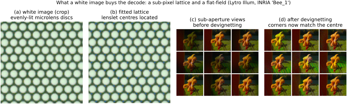
4. Refine the grid from a white image (sub-pixel). The metadata grid is good to a fraction of a pixel, but for clean output we fit the lattice to the data: blur the white image, find the bright center of every microlens disc near its predicted location, and least-squares-fit a full affine lattice (spacing, rotation, shear, center) to those centers. This affine fit improves the metadata grid (following the calibration approach of Dansereau, Pizarro & Williams 2013); it is not a full calibration of each ray through the main lens.
5. Resample to a uniform grid. For each microlens $(s,t)$ and each angular sample $(u,v)$, the corresponding sensor position is the microlens center plus a rotated angular offset; read it with bilinear interpolation (Chapter 6.5, Resampling and upsampling). This single gather turns the rotated hex sampling into an array whose Python axis order is (t, s, v, u, channel). Two subtleties decide the quality, both in From hexagonal lenslets to a uniform grid below: the angular offsets must span one lenslet, no more, and the hexagonal row stagger must be rectified.
6. Devignette (photometric flat-field). Each microlens images the main-lens aperture unevenly, so corner angular samples are darker and color-shifted: a per-$(u,v)$ vignetting. Decode the white image through the same grid into its own 4-D field and divide; because the white target is uniform, this flattens both the spatial and angular falloff. We divide by the white field's luminance (achromatic) so devignetting corrects brightness without re-tinting; white balance is a separate step. Achromatic division does not correct spatially varying color shading, and samples near the pupil boundary need particular care because dividing by a weak calibration signal amplifies noise. The implementation clamps the normalized flat field to 0.1 before division.
7. Color. White-balance, then apply the metadata color-correction matrix ccm (camera RGB → linear sRGB; its rows sum to 1, so it preserves neutrals). Do not use the metadata whiteBalanceGain directly (see Easy mistakes); it is in a Lytro-internal convention and does not neutralize the demosaicked RGB. The implementation derives gains from the white image or, lacking one, gray-world. A factory white image measures the calibration illuminant, however, not necessarily the scene illuminant. These gains do not guarantee neutral scene colors; use a neutral target under the scene lighting when color accuracy matters.
8. The result. Steps 1–7 produce a scene-linear 4-D light field. As in the DNG appendix, show it through a display tone-map (auto-exposure + gamma) only at the end: never bake the display curve into the array you will refocus or merge on.
raw, meta = imageio.imread(lfr)              # container parse + 10-bit unpack
lin   = (raw - black)/(white - black)        # 1: level correction (per Bayer channel)
rgb   = demosaic(lin, pattern="GRBG")        # 2: Bayer → RGB (full sensor res)
grid  = grid_from_metadata(meta)             # 3: hex lattice: pitch, rotation, offset
grid  = refine_from_white(white_raw, grid)   # 4: affine lattice fit to lenslet peaks
L     = build_lightfield(rgb, grid)          # 5: bilinear resample → L[s,t,u,v,c]
Lw    = build_lightfield(demosaic(white), grid)
L     = L / luminance(Lw).clip(eps)          # 6: achromatic devignetting
wb    = neutral_from(white) or gray_world(L) # 7: white balance (NOT metadata gains)
L     = clip((L * wb) @ ccm.T, 0)            #    colour-correction matrix → linear sRGB
# L is the scene-linear 4-D light field. Tone-map (gamma) is display-only.
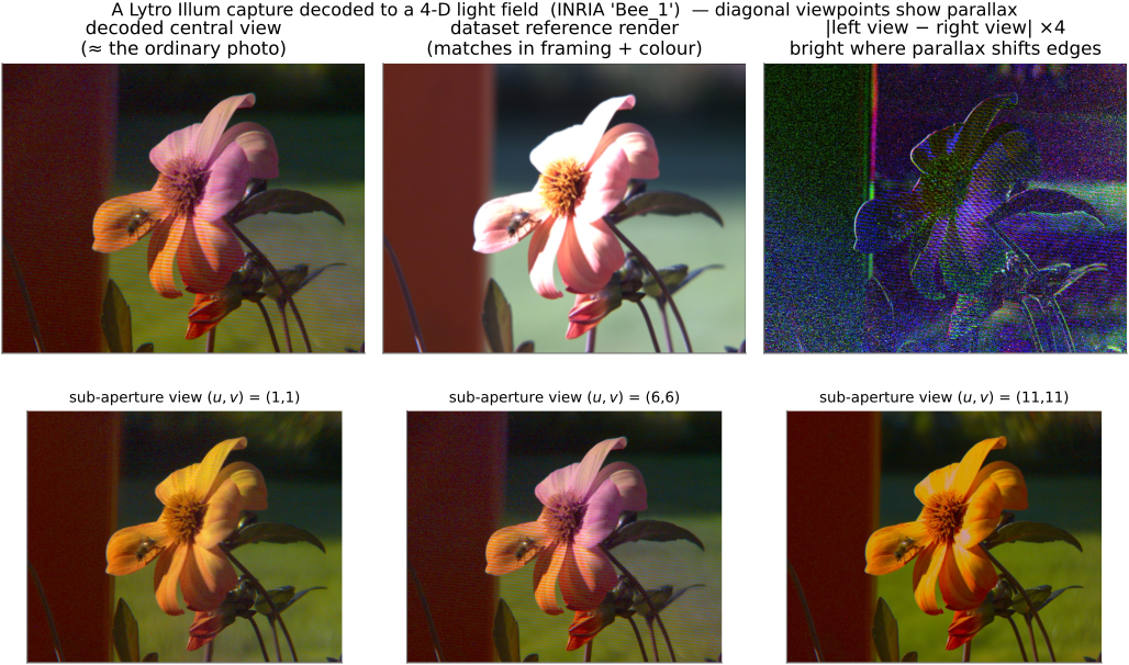
Array layout note: our code stores L[t, s, v, u, c] (spatial rows/cols, then angular rows/cols, then color), the book's $L(u,v,s,t)$ in a fixed index order. A sub-aperture view is L[:, :, v, u]; the central view is the all-but-pinhole photo at $(u,v)$ centered.
45.23.3 From hexagonal lenslets to a uniform grid⧉
This step has two common failure modes.
Angular span. Each microlens images the main-lens aperture onto a disc ~14 px across. The $(u,v)$ samples for that microlens must be read from within that disc. Span wider and you read into the dark gaps between lenslets and into the neighbors' discs: angular cross-talk that shows up as a halo or a color fringe at the edge of every sub-aperture view. We sample an odd $N\times N$ block (typically $13\times13$) with sample spacing equal to the pitch divided by $N$, rotated to match the array. The two extreme sample centers are therefore separated by $(N-1)/N$ of a pitch. The middle sample lands on the fitted lenslet center. A square block still has corners outside a circular pupil; those angular views need a pupil mask or confidence weights before quantitative use.
Hexagonal rectification. In a hex "row-major" array, alternate rows are offset by half a pitch. If you simply stack one sample per microlens into a rectangular array, the odd rows are shifted half a lenslet sideways from the even rows: a half-pixel comb that reads as fine horizontal banding on any smooth gradient. The fix is to resample the staggered rows onto a common column grid (interpolate the odd rows back by half a sample). This rectification approximates a rectangular spatial lattice. The implementation leaves the first column of staggered rows unchanged because it lacks a left neighbor; crop that boundary for methods that require uniform sampling. (This banding is geometric, not photometric: it is identical in a mono decode, which is how you tell it apart from vignetting.)
45.23.4 Why a white image⧉
A white image is a frame of a uniform, out-of-focus white surface: the target supplies approximately uniform radiance, while the variation within and across microlens discs reveals the lattice and measures vignetting. Its color response is a reference for the calibration illumination. The Lytro Illum ships a set of them (the dataset we use bundles 34, taken at assorted zoom and focus settings); the camera's caldata archive stores them as .RAW+.TXT pairs. The right one to use is the one whose zoom/focus matches the capture; our find_white_image picks it automatically by reading the zoom/focus steps from each white image's metadata. With it you get a sub-pixel grid (step 4), clean devignetting (step 6), and a color reference for the calibration illuminant (step 7); without it you fall back to the metadata grid and gray-world color, whose geometric and color errors depend on the capture.
45.23.5 Open questions and where we approximate⧉
Lytro is defunct, so unlike the DNG appendix we cannot ask the vendor; these are the places our decode is an informed approximation rather than a verified match.
- The color "look." We reproduce demosaic → white balance → color matrix faithfully, but Lytro's app applied an additional proprietary tone-and-hue "look" (as Lightroom does for DNGs, Chapter 45.15, Rendering a raw DNG — from sensor numbers to a faithful image). Our central views match the dataset's reference renders in geometry and overall color; exact hue/saturation may differ.
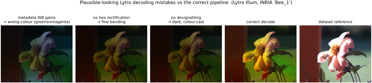
whiteBalanceGainconvention. The metadata gains do not neutralize the demosaicked RGB when applied as plain multipliers (they leave a strong cast: in our tests greens and magentas swap). We instead derive gains from the white image, with the scene-illuminant limitation described above. We do not know the exact stage/space those metadata gains are meant for.- Metadata grid vs white-image grid. For our camera the metadata pitch was accurate and only the center/rotation needed fitting; in general we trust the white-image affine fit. Whether the metadata grid is ever canonical we leave open.
45.23.6 Easy mistakes (most of which we made)⧉
A wrong light-field decode looks almost right. In rough order of how badly each bit us:
- Applying the metadata white-balance gains. The headline color bug. Multiplying by the metadata
whiteBalanceGainleaves a strong, wrong cast: greens and magentas swap (foliage goes magenta, flowers go yellow-green), and it looks plausible enough to ship. Our decoder uses the white image (or gray-world) instead; neither guarantees the correct scene white balance. We confirmed the demosaic was not the culprit by reading the raw Bayer phases directly. - "Fixing" color by swapping the Bayer pattern. Because the color looked wrong, the tempting move was to flip the mosaic (GRBG↔BGGR) until the flower looked pink. That is treating a white-balance bug as a demosaic bug; it leaves a subtler, scene-dependent cast. Verify the CFA from the raw data (which phase is brightest under a known-colored patch), then leave it alone.
- Forgetting the hexagonal stagger. Stacking one sample per microlens into a rectangular array without rectifying the half-pitch row offset gives a fine horizontal comb/banding. It is geometric (identical in a mono decode), so don't chase it in the color pipeline.
- Trusting the nominal lattice without a sub-pixel fit. A grid that is right on average but drifts a fraction of a pixel across the frame beats against the output grid and bands. Fit the lattice (center/rotation, and spacing in general) to a white image.
- Over-spanning the angular block. Reading $(u,v)$ samples wider than one lenslet pulls in the dark inter-lens gaps and the neighbors' discs: angular cross-talk, seen as haloed or fringed edges in the sub-aperture views.
- Demosaicking across lenslet boundaries, carelessly. The sub-images are separated by dark gaps; a demosaic that smears across them injects false color at every disc edge. (We demosaic the full frame but keep the lenslets large relative to the Bayer period, which keeps this mild; a lenslet-aware demosaic is the rigorous alternative.)
- Devignetting in color instead of luminance. Dividing the scene by the white field per channel both flat-fields and white-balances to the white image's illuminant, then applying white balance again double-corrects. Our pipeline devignettes by luminance and applies global white balance separately. A calibrated per-channel flat field is also legitimate, but its illuminant normalization and the later white balance must be designed together.
- Mismatched white image. Using a white image from the wrong zoom/focus mis-locates the lattice and mis-flattens the vignette. Match it by the zoom/focus metadata.
- Baking the display tone-map into the data. Saving gamma-encoded, tone-mapped views and then refocusing/merging on them does the math in the wrong space. The field you compute on is scene-linear; the tone-map is display-only (the thesis of Chapter 45.15, Rendering a raw DNG — from sensor numbers to a faithful image and Chapter 8.1, Image representation).