34.10 Ultra high-speed imaging🔗⧉

Light moves about 30 centimeters in a nanosecond, a billionth of a second, so to photograph light moving you need a camera whose shutter is sharper than a nanosecond. That is roughly a million times faster than the high-speed cameras that freeze a bullet or a popping balloon, and it is a different enterprise altogether. An ordinary high-speed camera runs the same kind of CMOS sensor we have studied, just read out very fast: thousands to a few million frames per second, enough to slow down a hummingbird, a splash, or a crash test. Those cameras belong with the rest of video and temporal sampling in Chapter 30.1, Motion blur, temporal sampling, and resampling. This chapter is about the regime past them, where the exposure is so short that the finite speed of light stops being instantaneous and becomes a signal you can record and exploit. At these timescales you can make a movie of a laser pulse sweeping across a scene, and more usefully, you can read the timing of light's bounces to recover depth, to see materials, and even to look around a corner.

To set scale: a sampling rate of a trillion (10¹²) frames per second places samples a picosecond apart; resolving events that close also requires an adequately narrow instrument response, the time light takes to cross a third of a millimeter. No electronic sensor can be read out that fast. The whole field is therefore a study in how to approximate an impossibly fast camera by sweeping time onto space, computing missing frames, or capturing the same ultrafast event many times.

34.10.1 Streak cameras: sweeping time onto a spatial axis🔗⧉

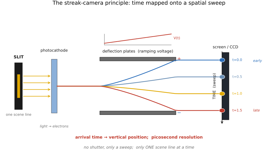
The foundational instrument is the streak camera, and its idea is to convert time into position so that an ordinary slow detector can record it. Light from a thin slit of the scene strikes a photocathode, which converts it to electrons; those electrons are accelerated through a fast-changing electric field, a deflection voltage that ramps during the event, so electrons arriving slightly later are bent slightly farther. They then hit a screen (or a CCD) at a position that encodes their arrival time. The result is a 2-D image with one spatial axis (along the slit) and one time axis (the sweep), with picosecond resolution along the time direction, an effective ultrafast temporal measurement, because it has no shutter, only a deflection that smears arrival time across the detector.

The cost is dimensionality: a streak camera images only a single line of the scene at a time (the slit), with the second image dimension spent on time. To get a 2-D movie you must recover the missing spatial axis somehow, which is the problem the next two methods solve, in opposite ways.

34.10.2 Femto-photography: a movie of light in flight🔗⧉

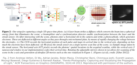
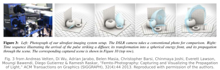
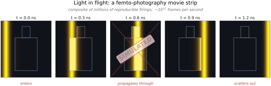
Femto-photography Velten et al. 2013 gets the missing spatial dimension by repetition. A laser fires ultrashort pulses, femtoseconds long, over and over, perfectly synchronized to a streak camera. For each firing the camera records one slit-line of the scene as the pulse's light washes across it, time-resolved to about two picoseconds. Scan the slit across the scene, line by line, accumulating over millions of identical laser shots, and you assemble a full 2-D image for each instant of time. Played back, the frames form a movie of light propagating, an effective rate around 10¹² (a trillion) frames per second, in which you can watch a pulse enter a scene, sweep across a wall, refract through a bottle, and scatter off into shadow. It is the most direct possible visualization of this chapter's premise: light is not everywhere at once; it travels, and here is the footage.

Two caveats keep the result grounded. First, it is not single-shot: the "movie" is a composite of millions of repetitions of an event that must be exactly reproducible, so it works for a controlled laser-lit scene, not for catching a one-time happening. Second, the propagation you watch is counterintuitive in subtle ways because the camera also obeys the speed of light, a wavefront can appear to move faster than light across the image, or backwards, depending on whether the light is heading toward or away from the lens. The footage is a real measurement, but reading it correctly takes care.

34.10.3 Compressive ultrafast photography: a single-shot coded streak🔗⧉

Femto-photography's limitation, needing millions of identical repetitions, is exactly what compressive ultrafast photography (CUP) Gao et al. 2014 removes, by capturing a genuinely non-repeatable, single-shot ultrafast event. The trick is to borrow from compressive sensing. Before the streak camera, the scene's full 2-D image is spatially coded with a pseudo-random mask, then the full two-dimensional coded image enters a streak system without the usual entrance slit. Time-dependent deflection shifts it along one detector axis, mixing that spatial coordinate with time. The recorded streak image is a scrambled, sheared mixture of all the space-time information: every spatial location and every time slice piled onto one frame. No single frame could hold a 2-D movie's worth of data, so the missing structure is recovered by computation: knowing the mask and the shear, a compressive-sensing reconstruction (an optimization using a sparsity or total-variation prior on a space-time volume consistent with the measurement) untangles the mixture back into a full 2-D movie, reported at up to ~10¹¹ frames per second from a single exposure. CUP is the encoding-and-solving cousin of femto-photography's repeat-and-scan: same goal, but it spends a clever optical code and a reconstruction algorithm instead of millions of reproducible shots, so it can reconstruct a one-time event consistent with that prior. The temporal sampling rate, effective resolution, noise, and reconstruction ambiguity are separate quantities. It is the same coded-measurement-plus-reconstruction philosophy that runs through coded aperture and coded exposure elsewhere in the book, pushed to the timescale of light.

34.10.4 Transient imaging and looking around corners🔗⧉

The streak-camera movie is only the start; the point is what the timing of light tells you about a scene. This is transient imaging: recording, per pixel, the full time profile of light arriving after a pulse, rather than just the total. That profile separates light by the path it took: light that went straight to a point and back arrives first; light that bounced off something else on the way arrives later, delayed by exactly the extra distance it traveled. Once you can time the bounces, indirect light stops being a nuisance and becomes a measurement of geometry you could not otherwise see.

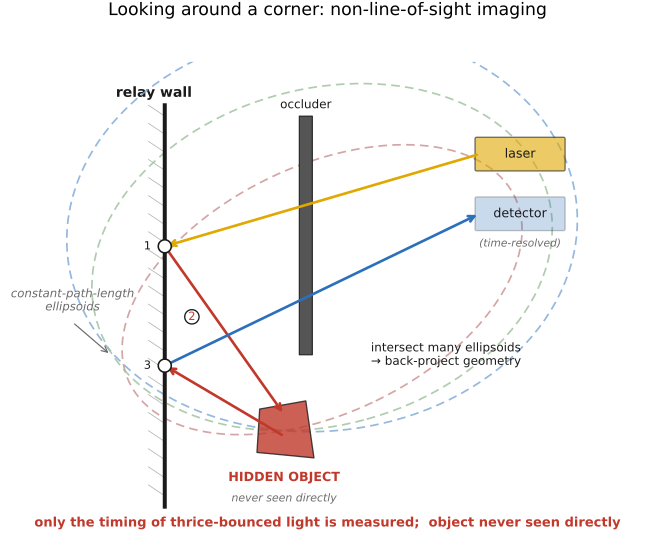
The signature result is non-line-of-sight (NLOS) imaging, looking around a corner Velten et al. (transient/NLOS). Aim an ultrafast laser and a time-resolved detector not at a hidden object but at a visible relay wall. A laser pulse hits the wall, scatters in all directions (the wall acts as a diffuse, room-sized "lens"), some of that light reaches a hidden object out of your direct line of sight, scatters again, returns to the wall, and finally bounces back to your detector. You never see the hidden object directly, only a faint, blurry glow on the wall, but you record precisely when each photon comes back. Each arrival time constrains the hidden object to lie on an ellipsoid (the set of points whose total bounce path matches that time-of-flight), and combining many such timing constraints, from many points on the wall, back-projects to reconstruct the hidden shape, the geometry around the corner, recovered from nothing but the timing of thrice-scattered light. It is the central result of transient imaging and a centerpiece of Part 38, Revealing the invisible: information that is completely invisible to an ordinary camera, dug out of the time domain.

34.10.5 The bridge to direct time-of-flight and LiDAR🔗⧉

All of this is the laboratory extreme of an idea that has become ordinary. Strip the streak camera and the femtosecond laser down to their essence: fire a pulse, time the return, range = ½ · c · time-of-flight, and you have direct time-of-flight LiDAR, the depth sensor in self-driving cars and recent phones and tablets (the depth-sensor and single-photon material of this part). The ultrafast-imaging methods here measure the whole time profile per pixel; a ranging LiDAR reports selected peaks or estimated ranges from its time measurements. Many systems retain multiple returns or histograms; the earliest detection can also be background noise rather than the desired direct return. And the detector that makes consumer single-photon LiDAR practical is exactly the single-photon avalanche diode of Chapter 34.5, Single-photon sensors (SPAD, avalanche, photon counting), a per-pixel picosecond stopwatch. So the chapter closes a loop: the same time-resolved sensing that lets a research rig watch light in flight and peer around corners, miniaturized and processed for ranging, is the rangefinder now riding in a phone. Capturing the timescale of light began as a way to see light itself and has become an everyday way to see depth.