30.1 Motion blur, temporal sampling, and resampling🔗⧉

The two great themes of spatial imaging are convolution (a measurement integrates over a region, the story of the point-spread function) and sampling (a discrete grid can only represent frequencies below its Nyquist limit, and anything faster aliases). This chapter makes one claim: both recur, identically, on the time axis. A photograph is not an instant; the shutter stays open for an exposure time, and the sensor integrates everything that lands during that window, so a moving scene smears, and motion blur is convolution in time. A video is not a continuous record; it is a sequence of frames at some rate, so motion faster than the frame rate folds down to a false, slow apparent motion, and temporal aliasing is the wagon-wheel effect, the temporal twin of moiré.

This matters because the two phenomena are one. The anti-alias filter you would want before sampling a video is a low-pass over time, and the camera already has one built in: the exposure window. Integrating over the exposure is the temporal prefilter, and the blur it produces is the price of suppressing aliasing. Motion blur and temporal aliasing are not two problems; they are the two outcomes of one knob, $\tau$. And the deeper question the chapter ends on (do I think of motion as particles I follow, or as a time-series at each fixed pixel?) is the Lagrangian vs Eulerian distinction, the frame that ties this whole part together.

30.1.1 A frame is an integral over time → motion blur🔗⧉

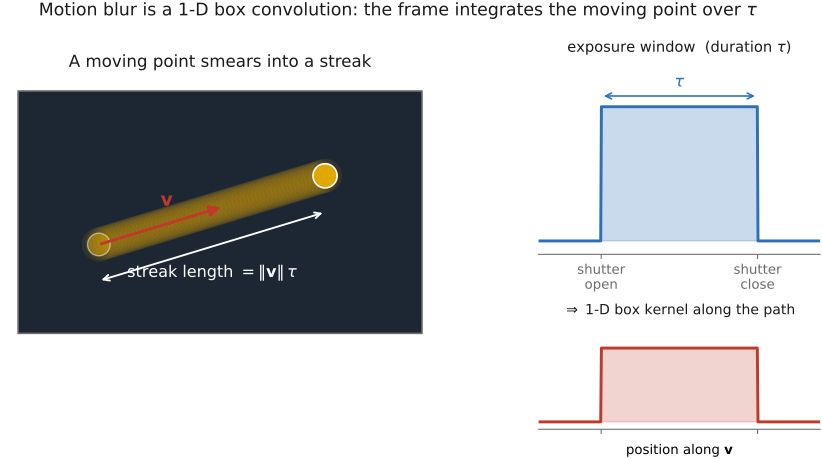
Start with the cause, intuition first. A photo is not a snapshot of a single instant. The shutter is open for an exposure time $\tau$, and over that whole window the sensor accumulates every photon that arrives. If a bright feature moves across the frame while the shutter is open, its light is deposited not at one place but along the entire path it travels, producing a streak rather than a point. Motion blur is precisely the temporal version of the standing intuition that a pixel is a weighted average of what it saw; here the average is taken over time rather than over a spatial neighborhood (Figure 30.1.4⛶ fullscreen).

Make it an equation. For an image-plane velocity $\mathbf v$, taken constant over the exposure, the blurred frame $B$ at pixel $\mathbf x$ is the time-average of the sharp scene $I$ over all the positions the scene occupied during the exposure:

Read it literally: the value recorded at $\mathbf x$ is the average of the sharp scene seen through a sliding offset $-\mathbf v t$, swept over the open-shutter interval $[0,\tau]$ and normalized by its length.

This integral is a convolution. Write it as

where the path kernel $k_{\mathbf v}$ is a 1-D box of length $\lVert\mathbf v\rVert\,\tau$, oriented along the motion direction $\mathbf v$, normalized to unit area. Constant velocity gives a straight box; curved motion gives a curved path kernel that traces the trajectory. This is the exact temporal analog of the spatial PSF. Spatial blur smears over a spatial neighborhood; motion blur smears over the motion path. It is the same operator (Chapter 6.7, Image formation as a linear system, now read in time), with the axis merely time projected onto space. Recall from the convolution material that convolution was the averaging / sum-of-random-variables operation in the first place; here the "random variable" being averaged is simply position-during-exposure.

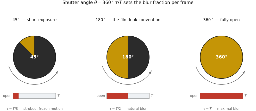
The photographer's knob for all of this is shutter speed, because the streak length is $\lVert\mathbf v\rVert\,\tau$ and so scales directly with exposure time. In cinematography the same control is expressed as a shutter angle,

the fraction of the frame interval $T$ that the (historically rotating-disc) shutter is open. The $180^\circ$ convention, $\tau = T/2$, gives the natural "film look"; $360^\circ$ integrates the whole interval and blurs maximally; small angles give crisp but strobed frames: the staccato, every-impact-frozen look of the Saving Private Ryan battle scenes (Figure 30.1.5⛶ fullscreen).

That sets up the tradeoff to state plainly. A longer $\tau$ collects more light, improving signal-to-noise, but produces more blur; a shorter $\tau$ gives sharper frames but less light and, as the next section shows, temporal aliasing. At a fixed frame rate and available light, exposure trades motion sharpness against photon collection and temporal filtering. It does not offer a universal rule that any two desired properties can always be achieved.

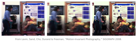
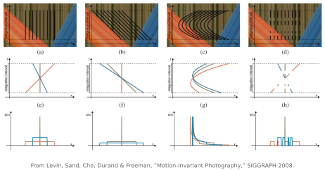
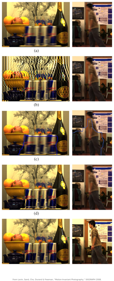
A forward-looking word on removing the blur. If the path kernel $k_{\mathbf v}$ is known, undoing motion blur is just deconvolution by it. But a straight-line box kernel has zeros in its frequency response, so naive inversion is ill-posed. This is exactly the Wiener / regularized-inversion story of Chapter 16.4, Blind deblurring, now with a motion PSF rather than a defocus one; when different objects move at different speeds the blur is spatially varying and no single kernel applies. One can even engineer the kernel to invert cleanly: a coded or "flutter" shutter (Raskar et al. 2006) chops the exposure open and closed to give $k_{\mathbf v}$ a broadband spectrum with better conditioning over the intended reconstruction band, and motion-invariant capture (Levin et al. 2008) sweeps the camera along a parabolic trajectory during the exposure so that motion along the designed direction has approximately the same PSF shape, up to a shift, over a supported range of velocities (Figure 30.1.1⛶ fullscreen, Figure 30.1.2⛶ fullscreen). The philosophy is the same "make the forward operator nice" move as coded aperture, and a single deconvolution by that one engineered kernel can sharpen objects within that motion model (Figure 30.1.3⛶ fullscreen).

30.1.2 Time is sampled → temporal aliasing, the wagon-wheel effect🔗⧉

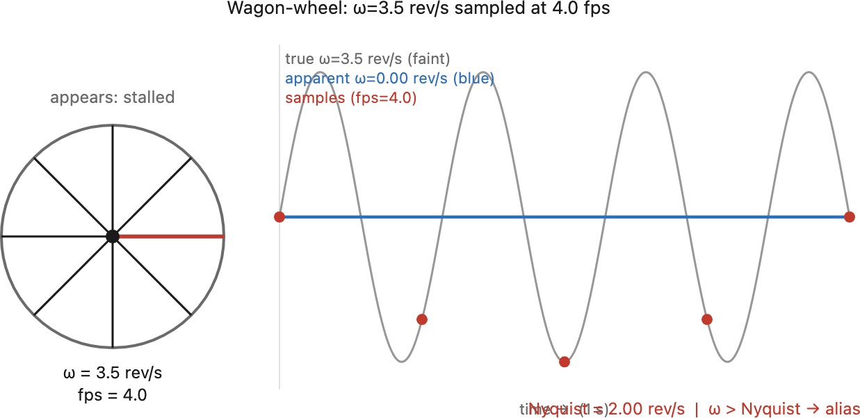
A video is a discrete sequence of frames at rate $f_s$: it samples the continuous motion of the world. And as with any sampling, motion components faster than half the frame rate cannot be represented and instead alias (the medium's temporal-sampling limit, Chapter 5.8, Photographic representation and its limits); they fold down to a false, slower, sometimes reversed apparent motion. This is L6.8show/L16 on the time axis.

The condition is the temporal Nyquist limit. To capture motion of temporal frequency $f_{\text{motion}}$ (say, a wheel's spokes passing a fixed point), you need

Violate it and the recorded apparent frequency folds to $f_{\text{app}} = \lvert f_{\text{motion}} - n f_s\rvert$, for the integer $n$ that brings the result into $[0, f_s/2]$.

The canonical demonstration is the wagon-wheel effect (Figure 30.1.6⛶ fullscreen). Film a spoked wheel at frame rate $f_s$. While the spoke-passing frequency stays below Nyquist the wheel turns forward correctly; as it climbs toward $f_s$ the wheel appears to slow, stall, then spin backward, because each frame catches the next spoke just short of where the previous one stood, so the sampled snapshots imply a small backward step per frame. It is the exact temporal twin of spatial moiré: undersampling maps a high frequency onto a wrong low one. Helicopter rotors and car rims under video or strobed streetlights show the identical artifact.

The everyday face of the same phenomenon is strobing / judder: fast pans, or fast subjects shot at low frame rate or with a very short shutter, look stuttery rather than smoothly flowing, because the motion is temporally undersampled and the eye perceives discrete jumps instead of continuous travel. Stroboscopic lighting that appears to freeze or reverse a spinning fan is the same effect, with the light doing the sampling instead of the shutter.

The fixes are the sampling toolkit, transplanted to time. One option is brute force: raise $f_s$. A higher frame rate buys a higher temporal Nyquist, which is exactly what high-speed cameras are for. The other is to prefilter before sampling, which on the time axis means integrate longer: a longer exposure is a wider temporal box, a low-pass that attenuates the offending high temporal frequencies before the frame grid samples them. And that prefilter is motion blur, which is why these two sections are really one story, the subject of the next.

30.1.3 Motion blur is the temporal prefilter: the two are one tradeoff🔗⧉

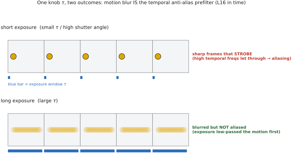
Here is the unification. The temporal anti-alias filter you would want in front of a video sampler is a low-pass over time, and the camera already supplies one: integration over the exposure window. A long exposure box-filters the motion in time before the frame rate samples it, suppressing exactly the high temporal frequencies that would otherwise alias. So motion blur and temporal aliasing are the two outcomes of one knob $\tau$: integrate more and you get blur (high temporal frequencies attenuated); integrate less and you get sharp frames that strobe (aliasing let through). They are not separate phenomena to be traded off against each other from outside. They are the two sides of a single dial (Figure 30.1.7⛶ fullscreen).

Why you cannot win for free is just the spatial L16 dilemma moved to the time axis: prefiltering buys freedom from aliasing at the cost of blur. The "right" exposure is a frequency-domain compromise: long enough to reduce unwanted high-frequency temporal content, short enough to keep the wanted motion sharp. Synthetic imaging faces the dual of this and resolves it the same way: computer-generated imagery (CGI) renderers add motion blur deliberately as a temporal anti-alias filter (Potmesil & Chakravarty 1983), integrating over sub-frame time samples so that fast on-screen motion blurs smoothly instead of strobing; the renderer is choosing a temporal $\tau$ exactly as a camera does.

There is an escape hatch, and it is the same one that recurs across the book: capture the full set, decide later. Shoot at a high frame rate with a short shutter (sharp and, if $f_s$ is high enough, alias-free), and then synthesize whatever motion blur or slow-motion you want afterward by integrating or interpolating frames. This defers the exposure-versus-blur decision out of the instant of capture entirely; it is the temporal cousin of capturing a light field and choosing the aperture later, and it sets up Chapter 30.4, Frame interpolation and slow-motion synthesis.

A box exposure is not an ideal temporal anti-alias filter. Its normalized frequency response has magnitude $|\operatorname{sinc}(f\tau)|$, with $\operatorname{sinc}(z)=\sin(\pi z)/(\pi z)$. It attenuates high frequencies but retains sidelobes above Nyquist, even when the exposure fills the frame interval. Increasing exposure can reduce aliasing without eliminating it. High-rate capture also retains a photon and bandwidth cost; later averaging cannot recover light that fell into gaps between exposures.

30.1.4 The film movie projector🔗⧉

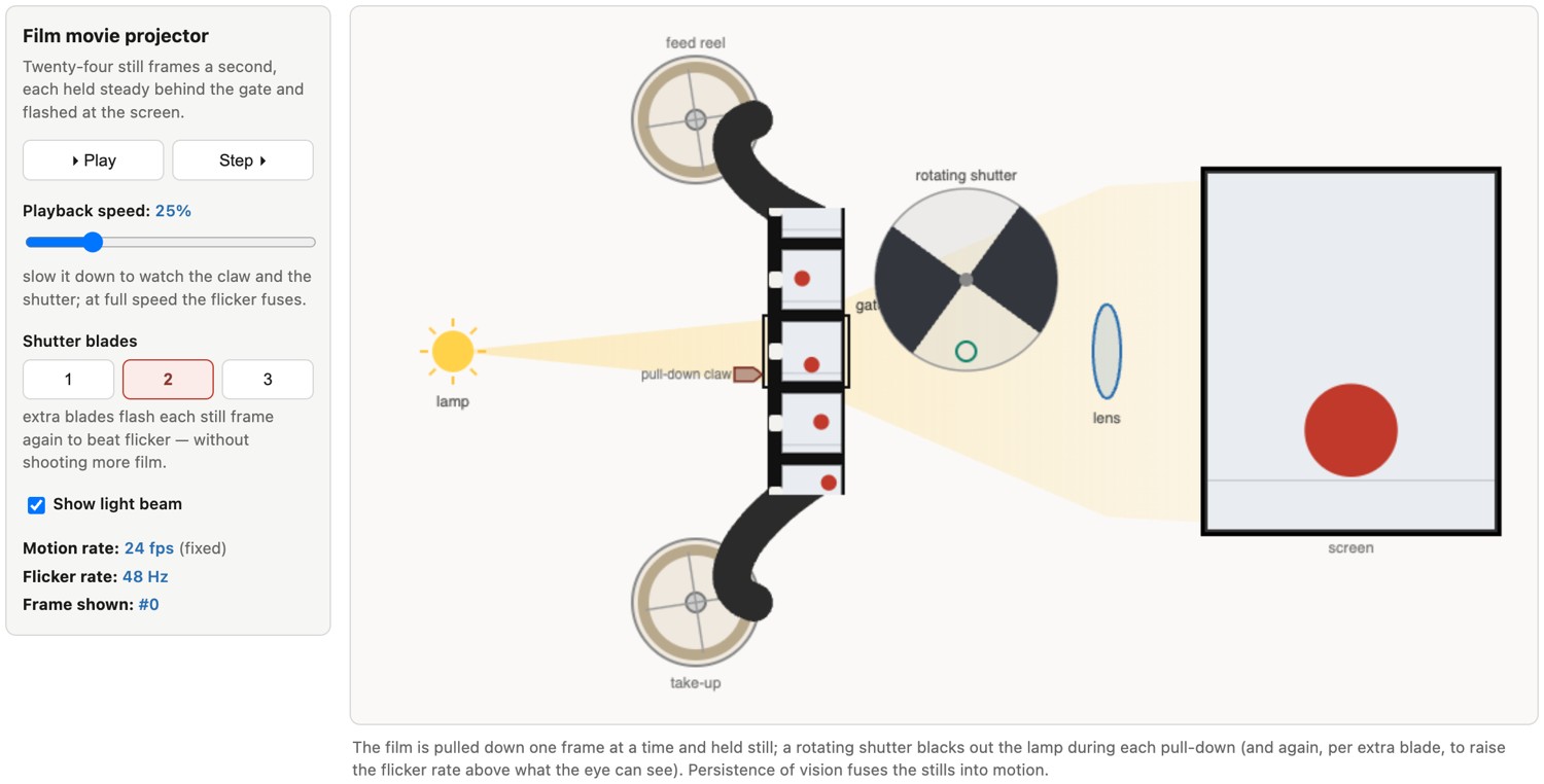
A film projector must move the strip between frames while holding it stationary for projection. Continuous reel motion is isolated from the intermittent gate transport by slack loops. Some systems use a claw, others an intermittent sprocket driven by a mechanism such as a Geneva movement. The shutter masks the transport so the moving strip is not projected as a smear.

At a film rate of 24 frames/s, flashing each stationary frame twice or three times produces 48 or 72 illumination pulses per second. There are still only 24 unique pictures. This separates motion sampling from flicker reduction: repeating a frame can reduce visible flicker without recovering intermediate object positions. Whether flicker remains visible depends on luminance, field size and viewing conditions. Apparent continuous motion is not adequately explained by “persistence of vision” alone.

The interactive mechanism links the temporal sampling model to a physical device. Compare changing the unique-frame rate with changing only the number of shutter interruptions per frame.

30.1.5 Resampling in time: frame-rate conversion🔗⧉

Once a video exists at one frame rate, showing it at another means resampling in time, and that runs into the same sampling laws. The classic case is broadcast. Film is shot at 24 fps, while television historically ran at about 30 fps (NTSC, really 60 interlaced fields per second) or 25 fps (PAL). Converting 24 to 30 fps cannot be done by copying frames evenly. The standard trick is 3:2 pulldown (telecine), which spreads four film frames across five video frames, in field terms a 3-fields-then-2-fields cadence. It lands the film on a 30 fps grid but adds an uneven, stuttering motion cadence known as telecine judder. PAL took a blunter route and simply played 24 fps film at 25 fps, a 4% speed-up that shortens the film and raises the audio pitch by nearly a semitone (the "PAL speedup").

The general problem is temporal resampling. Changing the frame rate means reconstructing the continuous motion signal and re-sampling it, so the rule from spatial resampling applies unchanged. Going to a lower rate needs a temporal prefilter, or the motion aliases and strobes; going to a higher rate needs interpolation between frames. Nearest-frame repetition gives an uneven or stepped motion cadence, while linear cross-fading can give ghosting, so motion-compensated frame interpolation estimates the motion and warps along it. That is how a modern television synthesizes 120 fps from a 24 or 30 fps source, and it is also what produces the smooth, hyper-real "soap-opera effect" many viewers dislike on film content, precisely because it removes the judder the cinematic 24 fps look depends on. Doing it well needs the full motion-estimation-and-warping machinery of Chapter 30.4, Frame interpolation and slow-motion synthesis. The point here is that frame-rate conversion is temporal resampling, subject to the same prefilter-then-sample discipline as every other axis in this book.

30.1.6 Lagrangian vs Eulerian: the organizing distinction for the part🔗⧉

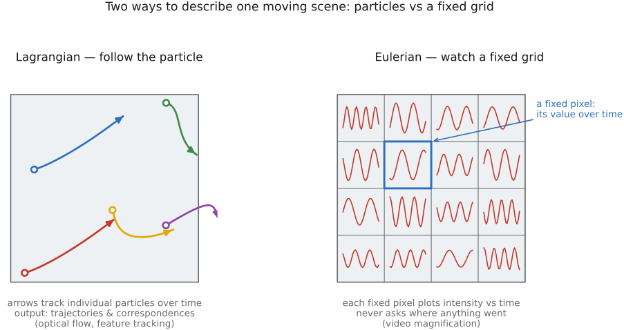
The last section introduces a distinction that frames the entire part. Borrowed from fluid dynamics, there are two ways to describe a moving scene, and almost every technique in this part commits to one of them.

The Lagrangian view says follow the particles. Attach yourself to a physical point in the scene and ask where it goes over time. This is tracking and optical flow: the output is trajectories and correspondences, a displacement field recording which point moved where, the material-derivative ($\tfrac{D}{Dt}$) way of looking at things.

The Eulerian view says watch fixed locations. Stay put at a single grid pixel and record the time series of intensity that passes through it. There is no correspondence, no "which point"; only what happened at this fixed cell over time. The output is a per-pixel signal in time (Figure 30.1.9⛶ fullscreen).

This is the right organizing axis because it cleanly sorts the part's methods and explains their difficulty. The Lagrangian methods are Chapter 12.8, Optical flow (dense, follow every pixel's motion) and Chapter 12.4, Feature tracking (sparse, follow distinctive points). They are hard precisely because correspondence is non-local and ill-posed: the aperture problem, occlusion, and large displacements all bite. Matching-based flow is "more Lagrangian" than differential flow exactly because it follows the patch rather than differentiating at a fixed pixel. The Eulerian method is video magnification (Chapter 38.3, Motion and video magnification), and its trick is to refuse correspondence altogether: take the time series at each fixed pixel, band-pass filter it in time, amplify the tiny temporal variations (a pulse in a cheek, a sub-pixel structural sway, a sound-induced vibration of a chip bag), and add them back. By never following particles, Eulerian processing sidesteps the entire hard matching problem; that is why it works on motions far too small to track. This chapter exists to set that contrast up.

The two views trade off against each other. Lagrangian gives you explicit, large-range correspondence: you genuinely know where the ball went. But you must solve the hard, ill-posed matching to get it. Eulerian is trivial to compute, just per-pixel temporal filtering, and excels at tiny, sub-pixel changes, but it has no notion of where anything went and breaks down for large motion, because a big displacement is simply not a small per-pixel perturbation. The rule of thumb: small motion → Eulerian; large motion → Lagrangian. (Phase-based magnification is a clever middle ground: Eulerian processing carried out in a steerable-pyramid phase representation, where local phase already encodes local motion.)