45.5 Problem Set 2 — Convolution and the bilateral filter⧉
Problem Set 2: Convolution and the Bilateral Filter. Due Wednesday September 30, 9:00pm.
45.5.1 Summary⧉
Important: This problem set is longer than the previous two. Reading the slides carefully can easily save you some headaches!
Image processing functions from the previous pset have been moved to basicImageManipulation.cpp and Image.cpp.
- brightness, contrast
- luminance, chrominance
- rgb2yuv, yuv2rgb
- gamma encoding, quantization
45.5.2 Smart Accessor⧉
When resampling images or performing neighborhood operations, we might end up accessing a pixel at x,y coordinates that are outside the image. To handle such cases gracefully, it is good practice to write accessors that take x,y as inputs and check them against the bounds of the image before retrieving a value.
Multiple options are possible when a pixel is requested outside the bounds; but the most common are to return a black pixel or the value of the closest valid pixel (i.e.\ of the closest edge). For the latter, clamp x to [0..width-1] and y to [0..height-1], and perform the lookup there.
Black padding (a.k.a.\ zero-padding) is more appropriate for applications such as scale and rotation (which we'll see in the next assignment) whereas edge-pixel padding generally looks better for convolution.
- 1 Implement
float Image::smartAccessor(int x, int y, int z, bool clamp=false) constinImage.cpp. The booleanclampallows you to switch between clamping the coordinates and returning a black pixel.
45.5.3 Blurring⧉
In the following problems, you will implement several functions in which you will convolve an image with a kernel. This will require that you index out of the bounds of the image. Handle these boundary effects with the smart accessor from Section Smart Accessor. Also, process each of the three color channels independently.
We have provided you with a function Image impulseImg(int k) that generates a $k \times k \times 1$ grayscale image that is black everywhere except for one pixel in the center that is completely white. If you convolve a kernel with this image, you should get a copy of the kernel in the center of the image. An example of this can be seen in in a2_main.cpp. It can also be useful to have simple images, such as an all white Image e.g. Image im(w,h,c); im.set_color(1.0, 1.0, 1.0);.
Box blur⧉
- 2.a Implement the box filter
Image boxBlur(const Image &im, int k, bool clamp=true)infiltering.cpp. Each pixel of the output is the average of its $k\times k$ neighbors in the input image, where $k$ is an integer. Make sure the average is centered. We will only test you on odd $k$ (that is the center of the filter is $[\frac{k-1}{2},\frac{k-1}{2}]$).- 2.b Can you think of ways to make the Box Blur filter computationally more efficient? (Answer in the submission form)
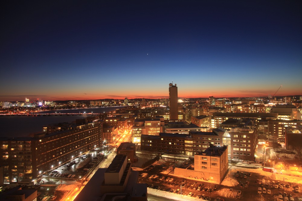
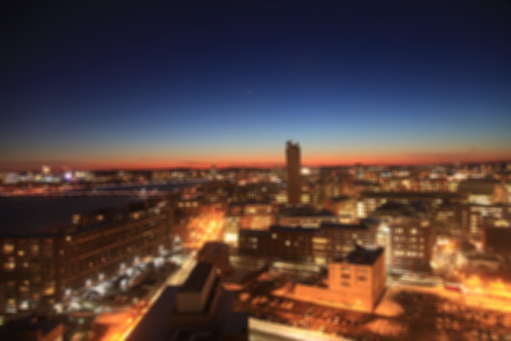
Figure 1. Result of blurring an image with a box width of k=9 and clamp=true
General kernels⧉
Now, let us implement a more general convolution function that uses an arbitary kernel. From now on, we'll perform this using the Filter class. This class contains a buffer of floats that represent the filtering kernel, together with its spatial footprint.
To create a filter use the constructor Filter(const vector<float> &fData, int fWidth, int fHeight). This takes in a row-major vector containing the values of the kernel (just like in the Image class), and the width and height of the kernel respectively (to avoid alignment and coordinate round-off issues, we'll use odd width and height). See a2_main.cpp for an example.
- 3.a Implement the function
Image convolve(const Image &im, bool clamp=true)in theFilterclass insidefiltering.cpp. This function should compute the convolution of an input image by its kernel. Make sure the convolution is centered.Note that the kernels are not flipped ahead of time. You may find the original format of convolution helpful, i.e. $(I\otimes g)(x)=\int_{x'}I(x')g(x-x')\mathrm{d}x'$. Tip: To access the
(x,y)location in a kernel from within the class typeoperator()(x, y).
- 3.b Implement the box filter using the
Convolvemethod of theFilterclass inImage boxBlur_filterClass(const Image &im, int k, bool clamp=true). Check that you get the same answer as before withboxBlur.- 3.c Create three small images of your own to use for testing and debugging your convolution code, and include them in your submission (see the naming scheme below). They should be images you construct, not photographs, and you should be able to predict by hand what comes out. For each one, say what the image is, why you chose it, which kernel you convolve it with, and what you expect the result to be. (Answer in the form)
Your test images.
Put the images you make in Input/debug/ and name them <part>_<n>_<what>.png, lowercase, at most $256\times256$ pixels: conv_1_… png to conv_3_… png here, and bila_1_… png to bila_3_… png later in the set. make prepare copies Input/debug/ into your submission, so they travel with your code. Write the filtered versions into Output/ under the same name with _out added, and keep the code that generates the images in a2_main.cpp.
Pay attention to indexing, $(0,0)$ denotes the upper left corner of the Image, but for our kernels we want the center to be in the middle. This means you might need to shift indices by half the kernel size. Test your function with impulseImg, a constant image and real images of your choice.
Gradients⧉
Image gradients measure the variation in intensity between neighboring pixels. We estimate gradients at each of pixel in the image using finite differences. Since this operation is identical regardless of the spatial location, we can write it as a convolution. A kernel often used to estimate the gradient is the Sobel kernel. Here are their weights(Note that the Sobel kernel is not scaled so that the output keeps the same range as the input, i.e. $[0,1]$. For visualizing image gradients, e.g. filtered results using a horizontal Sobel kernel as in Fig. 2(b), you might want to rescale the convolution output to [0,1] considering the possible output range convolved by this filter ($[-4,4]$ for the Sobel filter).) for the horizontal and vertical components of the gradient are respectively:
The gradient magnitude is defined as the square root of the sum of the squares of the two components(No need to rescale it to $[0,1]$, just keep it as the original range.) :
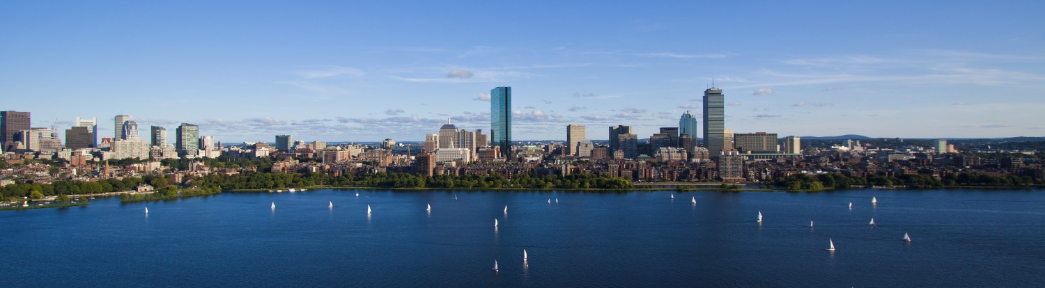
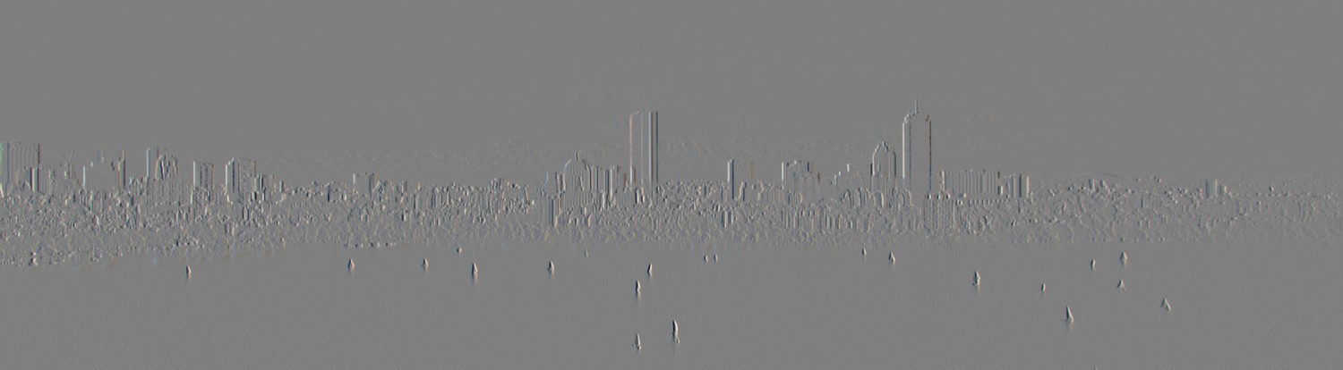
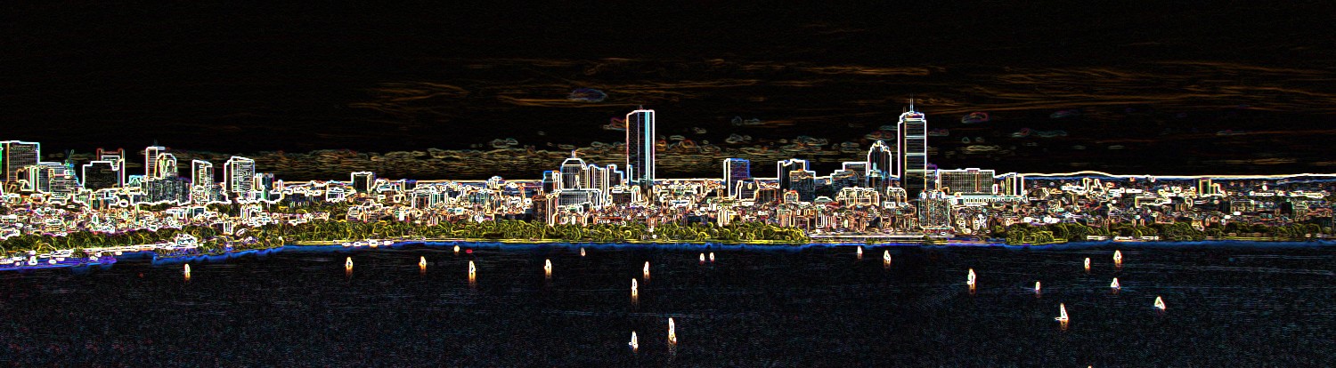
Figure 2. Result of filtering with a horizontal Sobel kernel and computing the gradient magnitude.
- 4.a Write a function
Image gradientMagnitude(const Image &im, bool clamp=true)that uses the Sobel kernel to compute the gradient magnitude from the horizontal and vertical components of the gradient of an image.- 4.b What kind of image structure does the gradient reveal? Can you imagine an application that would leverage this information? (Answer in the submission form)
Gaussian Filtering⧉
The Gaussian filter is ubiquitous in image processing. It is a key building block of many algorithms. We'll start by implementing a one-dimensional version of the Gaussian filter, then the 2D extension. The mathematical expression for a continuous normalized 1D Gaussian is:
Notice that $\frac{1}{\sqrt{2\pi \sigma^2}}$ is the normalization factor.
In practice, we will not care about this exact normalization factor since we are working with truncated and discrete Gaussians. Instead, we'll make sure our discrete filter is normalized, i.e. its weights sum to one.
1D Horizontal Gaussian filtering
- 5.a Implement
vector<float> gauss1DFilterValues(float sigma, float truncate)that returns the kernel values of a 1 dimensional Gaussian of standard deviationsigma. Gaussians have infinite support (they accept any $x$ from $-\infty$ to $\infty$), but their energy falls off so rapidly that you can truncate them attruncatetimes the standard deviationsigma. Make sure that your truncated kernel is normalized to sum to 1 and it is centered, where both sides of the Gaussian should be summed. Your kernel's output length should be1+2ceil(sigma truncate).- 5.b Use the returned vector from
gauss1DFilterValuesto generate a 1D horizontal Gaussian kernel using theFilterclass. Create and use thisFilterto blur an image horizontally inImage gaussianBlur_horizontal(const Image &im, float sigma, float truncate=3.0, bool clamp=true)- 5.c What is the effect on the output of varying sigma? (Answer in the form)
- 5.d How does
truncateimpact the computational cost? (Answer in the form)
2D Gaussian Filtering
Let us now extend our skinny 1D Gaussian to a the full-blown 2D version(Similar to the 1D case, $\propto$ means “proportional to” considering a normalization factor, which should be determined after truncation and discretization.), e.g.
- 6.a Implement a function
vector<float> gauss2DFilterValues(float sigma, float truncate)that returns a full 2D rotationally symmetric Gaussian kernel. The kernel should have standard deviationsigmacorresponding to a size of1+2ceil(sigma truncate)$\times$1+2ceil(sigma truncate)pixels.- 6.b Implement
Image gaussianBlur_2D(const Image &im, float sigma, float truncate=3.0, bool clamp=true)that uses the kernel fromgauss2DFilterValuesto filter an image.- 6.c How does the output differ qualitatively from the BoxBlur filter? (Answer in the form)
Separable 2D Gaussian Filtering
Filtering our images with a 2D Gaussian kernel gives us a nice blur effect, but it is computationally costly. Fortunately we can exploit the separability of the Gaussian kernel, and make the 2D convolution almost as fast as its 1D counterpart.
- 7 Implement separable Gaussian filtering in
Image gaussianBlur_separable(const Image &im, float sigma, float truncate=3.0, bool clamp=true), using a 1D horizontal Gaussian filter followed by a 1D vertical one.
Verify that you get the same result with the full 2D filtering as with the separable Gaussian filtering.
You can compare the running time of your two implementations following the example in the starter code in a2_main.cpp.
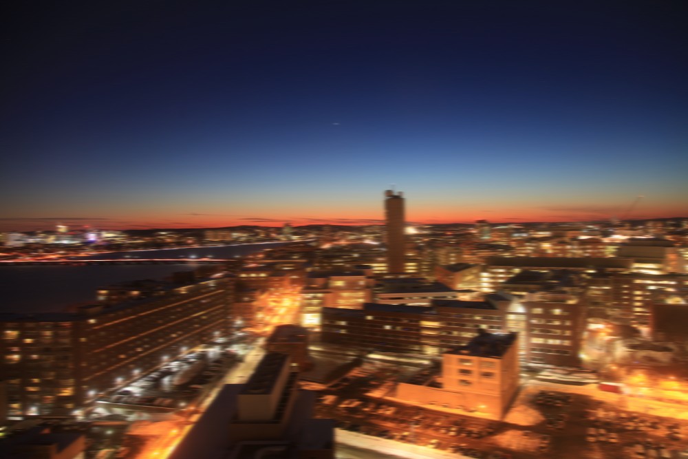
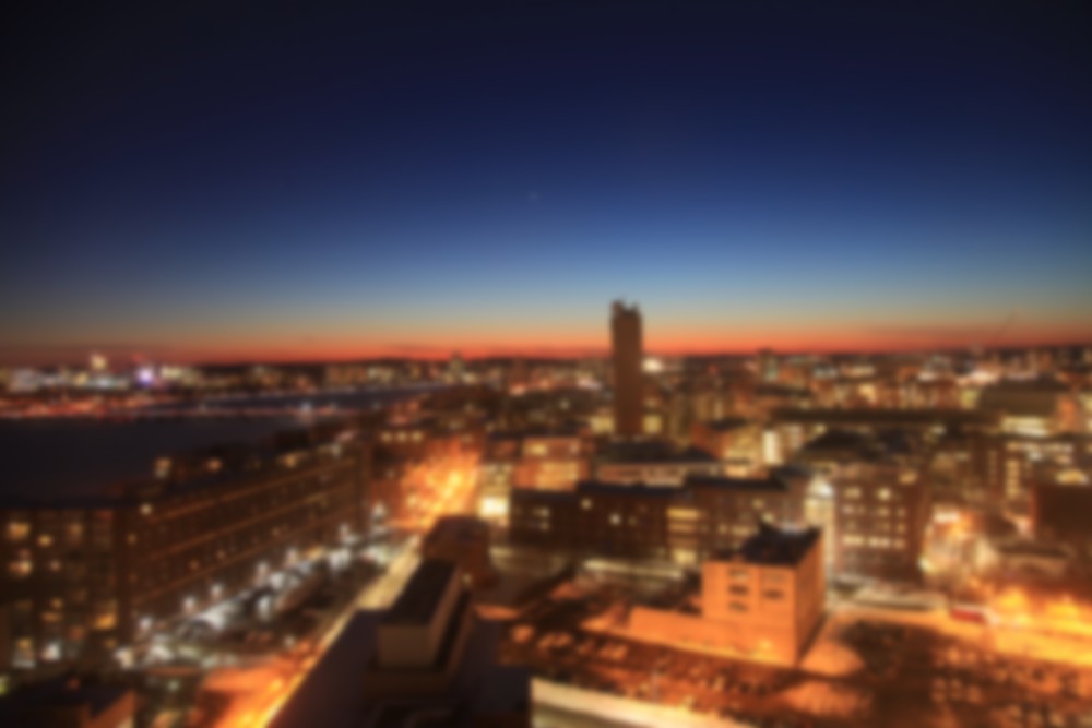
Figure 3. Result of blurring an image with a horizontal and 2D Gaussian kernel for sigma = 3.0, truncate=3.0, clamp=true
Sharpening⧉
- 8.a Implement
Image unsharpMask(const Image &im, float sigma, float truncate=3.0, float strength=1.0, bool clamp=true)to sharpen an image. Use a Gaussian of standard deviationsigmato extract a lowpassed version of the image. Subtract that lowpassed version from the original image to produce a highpassed version of the image and then add the highpassed version back to itstrengthtimes, that is$$ I_\mathtt{sharpen}=I+\mathtt{strength}\times(I-I\otimes g)\,. $$
- 8.b What is the influence of the strength parameter? How about sigma? How would you set sigma to emphasize very small-scale details? (Answer in the form)
45.5.4 Denoising using Bilateral Filtering⧉
The Bilateral filter is defined as:
where $I$ is the input image, $Z$ is a normalization factor and $G$ is a Gaussian kernel. The notation $G([x-x', y-y'], \sigma_D)$ is shorthand for $G(x-x', \sigma_D) \times G(y-y', \sigma_D)$. The bilateral filter is very similar to a convolution, but the “kernel” varies spatially and depends on the color difference between a pixel and its neighbors. The different standard deviations trade-off the spatial (domain), $\sigma_D$, and color differences (range), $\sigma_R$. It is important to note that unlike other kernels, the normalization here depends on the pixel values and cannot be computed ahead of time. The range Gaussian should be computed using the 3D Euclidean distance in RGB, that is $\|I(x,y) - I(x',y')\|$ above is a shorthand for $\sqrt{\sum_c (I(x,y,c) - I(x',y',c))^2}$ (loop over three color channels).
Warning: Because this is not a straightforward convolution, you will not be able to use the ${\tt Filter}$ class implementation for this part. The normalization process should proceed only once, that is ignoring it for each individual Gaussian kernels but applying it at the last step for all three color channels.
- 9.a Implement
Image bilateral(const Image &im, float sigmaRange=0.1, float sigmaDomain=1.0, float truncateDomain=3.0, bool clamp=true), that filters an image using the bilateral filter. Truncate the spatial Gaussian to a square window centered on the output pixel, of radiusceil(sigmaDomaintruncateDomain)and side2radius+1. The range Gaussian uses the distance over all three channels at once, so every channel of a pixel shares one weight, and neighbors outside the image come from your smart accessor, withclampdeciding what happens at the edge.- 9.b (extra) The Bilateral filter is often called an “edge-preserving” filter, do you have any intuition why that is? (Answer in the submission)
- 9.c Create three small images of your own to use for testing and debugging your bilateral filter, and include them in your submission, named
bila_1_… pngtobila_3_… pngunderInput/debug/as above. For each one, say what the image is, why you chose it, what parameters you run it with, and what you expect the output to look like. (Answer in the form)
Try your filter on the provided noisy image lens as well as on simple test cases (e.g. an image with a rectangle).
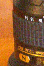
Figure 4. Results of denoising using a bilateral filter. RGB Bilateral Filtering: bilateral(im, 0.1,1.0,3.0,true); YUV Bilateral Filtering: bilaYUV(im, 0.1,1.0,4.0,3.0,true);
6.8370 only (or 5% Extra Credit): YUV version⧉
We want to avoid chromatic artifacts by filtering chrominance more than luminance. This is because the human visual system is more sensitive to low frequencies in the chrominance components.
- 10 Implement
Image bilaYUV(const Image &im, float sigmaRange=0.1, float sigmaY=1.0, float sigmaUV=4.0, float truncateDomain=3.0, bool clamp=true)that performs bilateral denoising in YUV where the Y channel gets denoised with a different domain sigma than the U and V channels. Convert the image to YUV and bilateral-filter the whole of it twice, once withsigmaYand once withsigmaUVas the domain sigma, so the two spatial radii areceil(sigmaYtruncateDomain)andceil(sigmaUVtruncateDomain). Keep $Y$ from the first result and $U$, $V$ from the second, compute the range weights over all three YUV channels as before, and return the image converted back to RGB.
In all cases, make sure you compute the range Gaussian with respect to the full YUV coordinates, and not just for the channel you are filtering. We recommend a spatial sigma four times bigger for U and V as for Y.
45.5.5 Extra credit⧉
Here are ideas for extensions you could attempt, for 5% each. At most, on the entire assignment, you can get 10% of extra credit:
- Median filter
- Summed Area tables (i.e. integral images) for faster box blur
- Different edge padding (e.g. mirroring)
- Fast incremental and separable box filter
- Use a look-up table to accelerate the computation of Gaussian values for bilateral filtering.
- Edge detection
- Smart sharpen (e.g. based on pixel value or edge detection)
- Difference of Gaussian with stylistic modifications <https://hpi.de/fileadmin/user_upload/fachgebiete/doellner/publications/2012/WKO12/winnemoeller-cag2012.pdf>
- Fast convolution using recursive Gaussian filtering:<http://citeseerx.ist.psu.edu/viewdoc/summary?doi=10.1.1.35.5904>
- Denoising using NL means <http://www.math.ens.fr/culturemath/maths/mathapli/imagerie-Morel/Buades-Coll-Morel-movies.pdf>
- Correcting for dark value bias in denoising (denoised images tend to be too bright because the negative component of noise is missing)
45.5.6 Submission⧉
Turn in your files to the online submission system and make sure all your files are in the asst directory under the root of the zip file. If your code compiles on the submission system, it is organized correctly. The submission system will run code in your main function, but we will not use this code for grading. The submission system should also show you the image your code writes to the ./Output directory
In the submission system, there will be a form in which you should answer the following questions:
- How long did the assignment take? (in minutes)
- Potential issues with your solution and explanation of partial completion (for partial credit)
- Any extra credit you may have implemented and their function signatures if applicable
- Collaboration acknowledgment (you must write your own code)
- What was most unclear/difficult?
- What was most exciting?