13.1 Noise models, transforms, and benchmarks🔗⧉

A denoiser configured for a noise standard deviation of 25 needs to know what those units mean. On an image scaled to $[0,1]$, the conventional 8-bit benchmark level is $25/255$, not 25. It also needs to know whether that level describes independent Gaussian noise, raw sensor noise, or the output of a camera pipeline.

Three kinds of intervention organize the whole problem. Improve the measurement by collecting more light or reducing electronic noise; acquire additional measurements that can be aligned and combined; or use assumptions about the clean image to resolve what one noisy observation leaves undetermined. Real cameras combine all three, and this part is mostly about the third.

Consider the hardware route first. A longer exposure can collect more photons, but a moving hand may blur. A larger collecting area can improve the photon budget under suitable capture conditions, but brings different size, cost, and optical tradeoffs. Reducing read noise helps especially when the signal is faint. These changes improve the measurement before a denoiser sees it. They do not recover a moving subject's lost sharpness or make saturation reversible; the capture tradeoffs are developed in Chapter 2.8, Noise, signal-to-noise ratio and dynamic range.

Additional measurements offer a different resource. Several aligned views of a still wall provide repeated noisy samples of the same underlying value. Averaging can reduce their independent fluctuations without assuming that the wall is spatially uniform. With one frame, averaging adjacent pixels instead assumes that those different locations ought to have similar values. That assumption is reasonable inside a uniform wall and wrong across its edge or fine texture. The numerical operation looks similar, but the source of its justification has changed.

The inverse-problem notation makes the distinction precise. For one frame, the forward operator is the identity: every location is observed, but its clean value remains uncertain. A noise likelihood still makes some candidate values more probable than others. Repeated aligned frames add observations of the same unknowns; an image prior instead relates those unknowns through assumptions about image structure. A burst method often uses both, since motion rejection, alignment, and weakly observed regions still benefit from an image model.

Those assumptions need not appear as a written probability distribution. Averaging a neighborhood assumes its underlying values are similar. Bilateral filtering Tomasi & Manduchi 1998 adds an assumption that value differences identify boundaries. Coefficient shrinkage uses the concentration of natural-image transform coefficients near zero. A learned denoiser takes its preferences from training examples and its architecture. Explicit statistical modeling makes some assumptions easier to inspect; learning them does not make them more appropriate for a particular camera.

Which route a camera can afford is an engineering decision. A viewfinder or video stream must deliver every frame within a deadline and sustain that work without excessive power or heat. A local filter can use a small row buffer and predictable work per pixel, making it attractive for a fixed-function image signal processor. A burst needs memory for multiple frames, alignment work, and enough agreement between their contents. It gains measurements but also has to handle a face or hand that moves between them.

A learned denoiser adds costs for its feature maps, weights, and arithmetic. An accelerator can make that computation practical, but its capacity and memory traffic still constrain the model and resolution. A still-image mode may accept latency that a live preview cannot. Consequently, one camera can use different combinations in preview, video, and final still processing. A learned stage also need not replace averaging: it can estimate alignment, reject inconsistent samples, combine a burst, or clean up the merged result. The useful deployment question is which measurements and computational resources are available for this mode, rather than which family is newest.

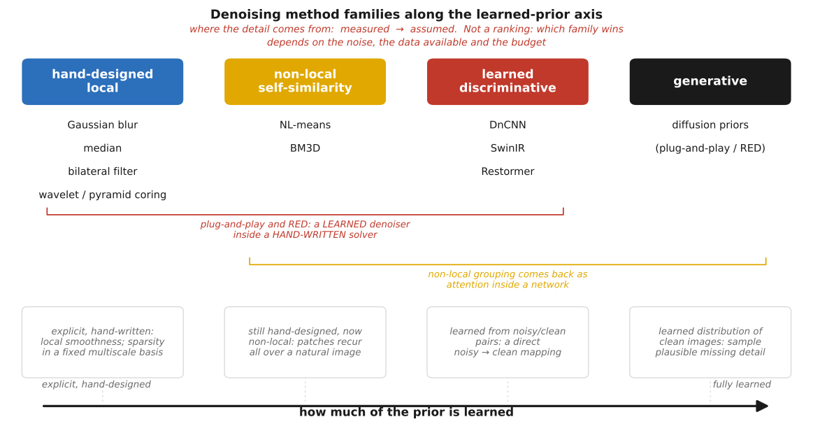
The sensor physics is developed in Chapter 2.8, Noise, signal-to-noise ratio and dynamic range. This chapter recalls the assumptions needed to use a denoiser and specifies what must accompany an experimental result. Figure 13.1.1⛶ fullscreen places the main method families beside their assumptions. Learning, non-local matching, and generative sampling are different design choices; they do not form a universal ranking of fidelity.

13.1.1 The noise that is actually there🔗⧉

Away from clipping, a black-level-corrected raw measurement can be modeled as

Here $x$ is the expected signal in raw-value units. The slope $a$ converts shot-noise variance into those units, and $b$ is the read-noise variance. Their values depend on the camera, gain setting, channel, and normalization. This variance law does not assert that the distribution is Gaussian: low-count shot noise remains discrete and asymmetric. The full Poisson/read-noise/clipping model and its simulator are given in Chapter 2.8, Noise, signal-to-noise ratio and dynamic range (Foi et al. 2008 (Poisson-Gaussian noise model)).

Estimate the noise curve from repeated static captures at fixed settings. For each sensor position, measure the mean and temporal variance, then fit variance against mean. Use unclipped values, stable illumination, and consistent color-filter channels. Camera motion must be negligible; interpolation during registration changes the noise being measured. Figure 13.1.2⛶ fullscreen illustrates the fit.

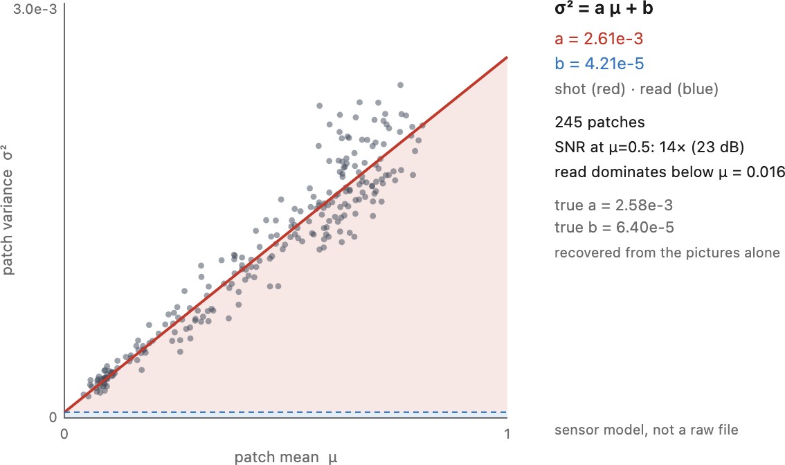
The affine law is why noise is a problem of the shadows rather than the highlights. Shot noise grows with brightness in absolute terms, since its standard deviation is the square root of the collected count, but it grows more slowly than the signal does, so the ratio improves with light. A bright pixel carries the most absolute noise and the best ratio; a dark pixel carries little absolute noise and a poor one, and the eye reads the ratio. Read noise, a fixed additive term, sharpens that contrast by dominating exactly where the light is faintest.

Two practical routes to the numbers. A burst of a static scene on a tripod gives the temporal spread at each pixel directly. A pair of flat-field captures gives it spatially: difference the two frames and divide by $\sqrt2$, which removes the shared scene and the fixed response, provided the pair is aligned and the two noise draws are independent.

A guard belongs with any variance estimate that something later divides by. A perfectly flat patch, a saturated one, or a patch of a few identical values can return an estimated variance of exactly zero, and every weight of the form $1/\hat\sigma^2$ then becomes infinite: the estimator hands the whole average to one sample, or the code raises. Clamp the estimate to a small positive floor, $\max(\hat\sigma^2,\varepsilon)$ with $\varepsilon$ in the units the estimate is in, and read a patch that reaches the floor as a measurement that failed rather than as a noiseless one. The same guard applies to a per-pixel variance map computed from a short burst, where a handful of frames makes zeros common.

A single-frame estimate from flat patches is possible, but scene texture and spatial response variation also contribute to spatial variance. Low gradient alone does not establish that a patch contains only noise. The burst procedure separates temporal variation from a fixed scene more directly.

Before choosing a method, identify departures from the model. Fixed-pattern offsets need calibration. Row or column fluctuations produce correlated noise. Demosaicking mixes neighboring measurements and correlates their errors. A model trained for independent noise may mistake these structures for signal; a method trained or designed for correlated noise can treat them explicitly. Black-level subtraction must preserve small negative values, as explained in the noise chapter.

Here is a calibration procedure using repeated captures. Unlike the spatial variance of a single patch, temporal variance compares the same sensor position across independent exposures of a static scene. Fixed spatial texture contributes to the mean image rather than to the temporal fluctuations.

import numpy as np

def fit_noise_curve(frames, valid):
    # frames: (number_of_captures, height, width), one CFA channel,
    # black-level corrected, finite, identically scaled and unregistered.
    # valid: mask excluding clipping, defects and unstable illumination.
    frames = np.asarray(frames, dtype=np.float64)
    if frames.ndim != 3 or frames.shape[0] < 2:
        raise ValueError("at least two repeated captures are required")
    mean = frames.mean(axis=0)
    variance = frames.var(axis=0, ddof=1)
    mu = mean[valid]
    vv = variance[valid]
    if mu.size < 2 or np.ptp(mu) == 0:
        raise ValueError("calibration needs a range of mean signals")
    a, b = np.linalg.lstsq(np.column_stack([mu, np.ones_like(mu)]),
                          vv, rcond=None)[0]
    return a, b

This ordinary least-squares fit illustrates the measurement. With few captures, individual variance estimates are noisy; pooling comparable sites or repeating flat-field measurements at several illumination levels improves the estimate. A negative fitted coefficient is a reason to inspect the calibration, not evidence of negative physical noise variance. Check residuals against mean and sensor position before trusting a single affine model.

A row offset is a different error from independent noise at each photosite. If every pixel on a row fluctuates upward together, averaging along that row preserves the fluctuation instead of canceling it. A denoiser that removes small independent variations can even make the remaining stripe easier to see. Calibration pixels or repeated captures can help distinguish a sensor-coordinate pattern from scene structure, but estimating a row offset from the scene risks removing a real horizontal feature. The correlation model determines which samples provide independent evidence.

ISO invariance affects what the denoiser receives. At fixed aperture and exposure time, changing analog gain does not collect more photons. If downstream readout and quantization errors are already small, brightening a lower-gain raw capture can give similar shadow quality to a higher-gain capture while retaining more highlight headroom. This is a sensor- and setting-dependent comparison, not a reason to reduce photon exposure without cost. Conversion-gain switches can change read noise abruptly, so calibrate each operating mode rather than fitting one curve across ISO settings. Chapter 2.8, Noise, signal-to-noise ratio and dynamic range develops that capture-side distinction.

13.1.2 Choosing the working domain🔗⧉

For a raw pipeline we use black-level-corrected linear values and a noise model calibrated in the same units. This keeps the connection to photon counts explicit. Denoising a processed image is also possible, but the model must describe that processed image.

A nonlinear encoding changes the variance. For a smooth encoding $g$ and small fluctuations around $x$, a first-order expansion gives

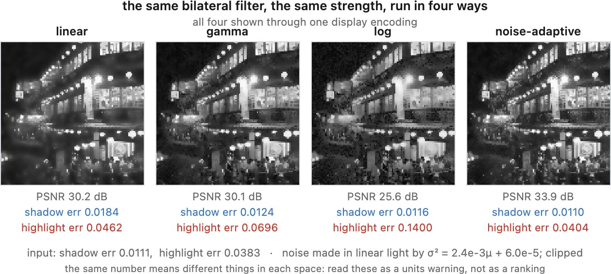
The local slope of the encoding scales the noise standard deviation. A compressive curve has a smaller slope in highlights than in shadows, so it changes their noise scales differently. This explains the approximate stabilization discussed in Noise, signal-to-noise ratio and dynamic range#Making noise variance uniform. It does not make a fixed filter strength interchangeable between linear, gamma, and log values (Figure 13.1.3⛶ fullscreen).

Decoding a JPEG reverses its known display encoding; it does not undo demosaicking, earlier denoising, clipping, compression, or an unknown local tone map. Use a denoiser intended for that input domain. In either domain, distinguish the statistical noise level from a user-selected amount of smoothing.

A gain changes both signal and noise units. If $z=cy$ for a known positive gain $c$, then $x_z=cx$ and $\operatorname{Var}(z\mid x_z)=ca x_z+c^2b$. Thus the shot-noise slope scales by $c$ and the read-noise variance by $c^2$. Apply this conversion to white-balance and lens-shading gains before passing a noise map to a model.

13.1.3 Variance-stabilizing transforms🔗⧉

The Anscombe transforms from Noise, signal-to-noise ratio and dynamic range#Making noise variance uniform let a constant-variance Gaussian denoiser operate on approximately stabilized sensor data. For Poisson counts, $f(y)=2\sqrt{y+3/8}$. For calibrated Poisson-Gaussian data, use its generalized form with the same gain and read-noise units as the measurement (Anscombe 1948 (variance-stabilizing transform)).

The intuition follows from the derivative. Ignoring the small-count correction, $f'(x)=1/\sqrt{x}$, so Poisson variance $x$ becomes approximately $(1/\sqrt{x})^2x=1$. A count near 100 has standard deviation 10 and transform slope about $1/10$; near 10,000 these become 100 and $1/100$. Both transformed standard deviations are about one.

Denoising estimates a clean transformed value, so the final step needs a bias-corrected inverse rather than simply squaring the estimate. Mäkitalo and Foi provide exact unbiased inverses and practical approximations (Mäkitalo & Foi 2013 (generalized Anscombe)). Clipping and parameter mismatch require separate care; stabilization does not recover missing measurements or guarantee Gaussian statistics at very low counts.

z = generalized_anscombe(y, calibrated_noise_parameters)
z_est = gaussian_denoiser(z, noise_std=1)
x_est = bias_corrected_inverse(z_est, calibrated_noise_parameters)

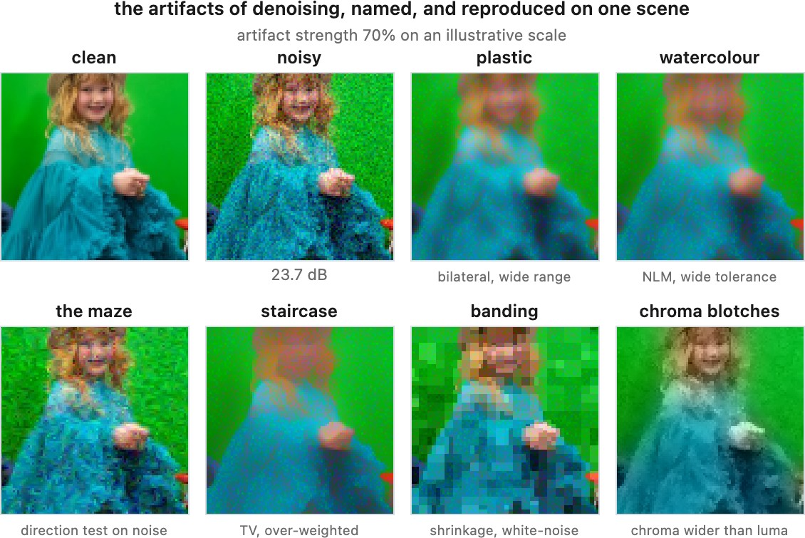
Check the output for lost texture, false contours, and remaining structured noise. Figure 13.1.4⛶ fullscreen collects examples that will recur in the algorithm chapters.

The inverse matters because the denoiser has changed the statistical object being inverted. Transforming each noisy observation and averaging is not generally the same as transforming the clean mean. Applying the algebraic inverse to that average can therefore retain a bias, especially at low counts. A bias-aware inverse accounts for the forward transform's noise statistics rather than merely undoing its formula. This distinction remains even if the denoising in the transformed domain is effective Mäkitalo & Foi 2013 (generalized Anscombe).

13.1.4 A ladder of difficulty🔗⧉

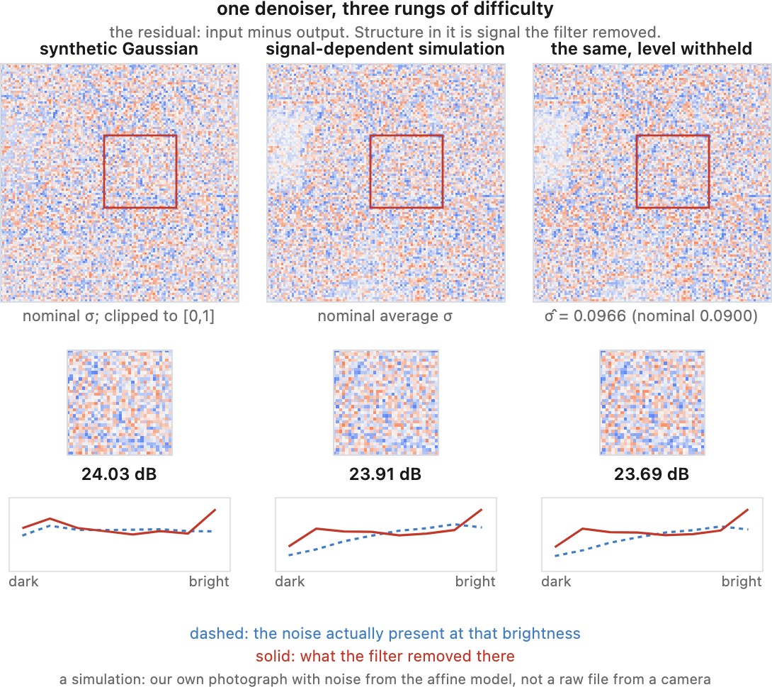
A paper's input assumptions determine which problem its score describes:

1. Known additive white Gaussian noise (AWGN). Add independent Gaussian errors with a stated standard deviation to a clean image. Specify its scale and whether the noisy input was clipped. Clipping changes both the distribution and the estimation problem.
2. Calibrated real noise. Supply sensor measurements and a known noise model or metadata. Signal dependence, clipping, and correlations may matter even when their parameters are available.
3. Blind denoising. The method must estimate the noise level or structure as well as the clean image. A network trained across unknown Gaussian levels solves a narrower blind problem than one intended for arbitrary processed photographs.

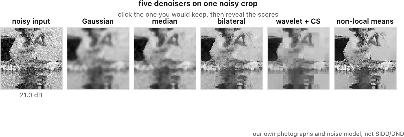
These are useful experimental distinctions, not a strict ordering of every dataset by difficulty. A textured low-noise scene can be harder for one method than a flat high-noise scene. Compare methods under the same available information (Figure 13.1.5⛶ fullscreen).

13.1.5 Salt and pepper is a different problem🔗⧉

Impulse corruption replaces a small fraction of measurements by extreme values. For example, a defective pixel may remain bright in every frame. The remaining pixels can still carry ordinary shot and read noise. The classical salt-and-pepper model replaces selected values by black or white; it is a contamination model, not necessarily a heavy-tailed distribution in the strict probabilistic sense.

An extreme sample can move the mean substantially. The median is less sensitive to its magnitude, provided fewer than half the samples in the neighborhood are corrupted and the clean signal is sufficiently constant there. At a narrow line or an isolated highlight, the same median can remove a real feature. Chapter 13.3, Gaussian, median, and bilateral filtering develops this tradeoff.

Use a calibrated defect map when available. A dedicated impulse-removal stage can prevent a bad pixel from spreading during demosaicking, but it should distinguish persistent sensor defects from real small bright objects.

13.1.6 Benchmarks, and what a leaderboard number means🔗⧉

SIDD, the Smartphone Image Denoising Dataset, provides repeated smartphone captures and carefully estimated clean references (Abdelhamed, Lin & Brown 2018 (SIDD)). DND, the Darmstadt Noise Dataset, uses low-noise references and intensity alignment for real camera photographs (Plötz & Roth 2017 (DND)). Both support evaluation in raw and processed color domains. The way each was built is instructive. SIDD photographed ten static scenes with five smartphone cameras under several lighting conditions, and estimated each clean reference from a long sequence of frames of the same scene, after correcting for misalignment and defective pixels. DND paired each noisy high-ISO photograph with a low-ISO, longer exposure of the same static scene from four consumer cameras, then corrected the residual intensity and alignment differences between the two. Both designs rely on a static scene and a fixed camera, which is why neither contains motion. Their references are estimates obtained from captures, not exact noise-free access to the scene.

Always identify the dataset version, split, input domain, and scoring protocol. Raw-domain and sRGB scores answer different questions. Hold out scenes when testing generalization to new content; hold out cameras when claiming generalization to new sensors. A private test reference reduces direct access to test targets but does not prevent overfitting through repeated submissions.

PSNR measures squared reconstruction error, while SSIM compares local image structure (Chapter 9.3, Image metrics). Under squared-error training, the population-optimal estimator is the conditional mean; uncertain fine detail can therefore be smoothed. A higher score does not establish that a method preserved every photographic feature. Conversely, more visible texture does not establish that the texture is correct. Compare the image, the error against the reference, and the removed signal, using a common display transform (Figure 13.1.6⛶ fullscreen). Chapter 13.12, Measuring a denoiser specifies the full evaluation procedure.