14.10 Video super-resolution and practical systems🔗⧉

Neighboring video frames can add sampling diversity and reduce uncertainty, provided that they observe corresponding scene content. Motion blur, compression and occlusion can make those frames less useful than a still-image model expects.

Video also imposes latency and temporal-stability constraints. A long clip does not give each region arbitrarily many useful measurements: content leaves the frame, changes appearance, or becomes occluded.

14.10.1 Temporal consistency is the new constraint🔗⧉

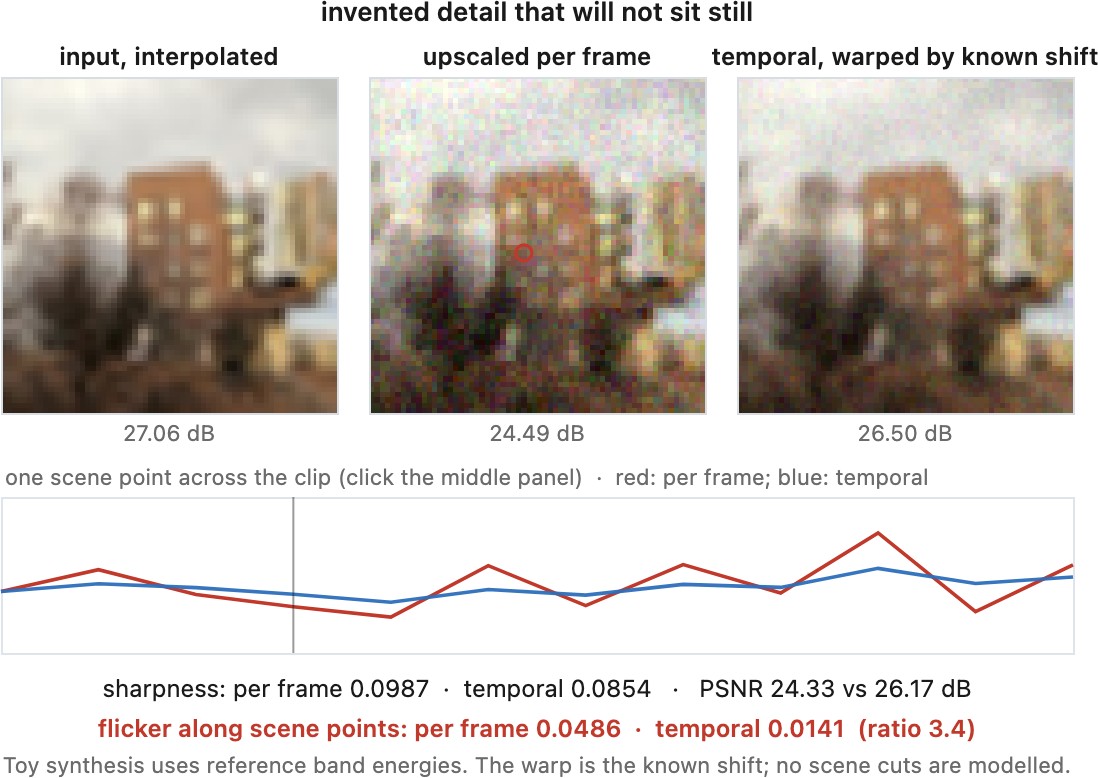
Independent per-frame processing can cause changing texture, edge sharpness or artifacts. View the output at its intended frame rate and inspect scene cuts as well as slow motion.

Small changes in motion, noise and sampling phase can change a deterministic network's output as well as a stochastic sampler's. These changes are not necessarily independent across frames.

Generative reconstruction must handle temporal conditioning explicitly when its outputs vary over time. Flicker is not unique to hallucination: ordinary resampling, correspondence errors and changing denoising strength can also produce it.

Framewise PSNR records errors in individual frames but does not characterize their temporal structure. Add playback and motion-compensated diagnostics with common validity masks, as in Chapter 13.10, Video denoising.

14.10.2 Using the neighbors🔗⧉

Three ways of bringing information from the other frames, in the order the field tried them.

Explicit alignment. Estimate optical flow to the reference frame, warp the neighbors, and feed the aligned stack to a network. This is Chapter 14.2, Multi-frame super-resolution's formulation with a learned reconstruction, and it inherits its weakness: flow errors put real content in the wrong place, and the network must learn or be given confidence cues to reduce those errors.

Implicit alignment. Deformable convolutions let the network learn per-pixel sampling offsets rather than being handed a flow field, so alignment becomes part of what is trained. EDVR (Wang et al. 2019 (EDVR)) is the reference point, with alignment done in a pyramid and a fusion stage that weights each frame per pixel, which is the robust merge of the burst chapter appearing again as a learned module.

Recurrence. Carry a hidden state from frame to frame, warping it forward (Sajjadi, Vemulapalli & Brown 2018 (frame-recurrent VSR)), so the effective number of frames contributing to any output grows without a growing window. BasicVSR (Chan et al. 2021 (BasicVSR)) made the case that a simple bidirectional recurrent design with good alignment beats elaborate architectures, and its successor added a propagation scheme that is more robust to occlusion. Bidirectional propagation is offline by construction, since it needs frames from the future; a live system needs a separately designed or trained causal path, or a bounded future window with declared delay. Simply deleting half of a trained bidirectional model need not work.

# recurrent video super-resolution, forward pass
prev_y = None
h = zeros(state_shape)                       # accumulated evidence, at low resolution
for y in frames:
    if prev_y is None or scene_cut(prev_y, y):
        h = zeros(state_shape)
        d = zeros(flow_shape)
        valid = zeros(mask_shape)
    else:
        d = target_to_source_flow(target=y, source=prev_y)
        h, valid = sample_source(h, grid + d)                           # bring the state into this frame
    c = confidence(h, y, d) * valid                  # occlusion and flow failure gate it
    h = fuse(h, feat(y), c)                  # accumulate; c decides how much to trust history
    x = pixel_shuffle(upsample_head(h), r)   # decode only at the end, as in the still case
    emit(x + upsample_bicubic(y))
    prev_y = y

14.10.3 Hybrid space-time super-resolution🔗⧉

The burst idea generalizes to the time axis, and once it does, spatial detail and temporal sampling can complement one another under a suitable motion model.

Motion is what makes the trade possible. An object crossing the sensor is sampled at a slightly different sub-pixel position in every frame, so its own movement supplies the staggered sampling that hand tremor supplies in Chapter 14.2, Multi-frame super-resolution. Several captures that are coarse in space and fine in time can therefore be combined into one that is finer in space, along the direction of motion. The exchange runs the other way too: a stack of high-resolution but slow frames, combined with the motion estimated from a fast low-resolution stream, reconstructs high-resolution frames at the fast rate, which is temporal super-resolution paid for in spatial samples.

The hardware version of the same argument is a hybrid camera, a fast low-resolution sensor and a slow high-resolution one looking at the same scene through a beam splitter. The fast one measures motion and short-timescale events; the slow one measures detail; and the reconstruction fuses them into something neither could capture. Such a rig requires its own geometric, temporal and radiometric calibration; it is not the capture setup of every burst dataset.

What limits it is what limits every method in this part. The extra spatial constraints depend on how much new sampling the motion provides. Steady motion can supply distinct phases along its direction; a static scene with a fixed camera repeats the same positions, so those frames reduce noise without adding sampling phases. And the motion has to be estimated accurately enough to place those samples, which is the registration problem of Chapter 14.2, Multi-frame super-resolution with a moving subject rather than a moving camera, and therefore harder.

14.10.4 What is deployed🔗⧉

Rendering systems such as DLSS use low-resolution frames, jitter and renderer-supplied motion data. This gives information unavailable to a camera, but does not make correspondence perfect: reflections, transparency, disocclusion and effects without valid motion vectors still require special handling. NVIDIA's DLSS 4 technical account discusses these limits.

Upscaling in streaming trades transmitted detail against bitrate and receiver computation. Editing tools enlarge individual photographs; their usefulness depends on output size and fidelity. Neither use has one universal tolerance for reconstructed text or faces.

Google's 2025 description of Pro Res Zoom identifies diffusion-based processing on Pixel 10 Pro and Pro XL and a zoom range reaching 100x (Google "Pro Res Zoom" 2025). This is a product-specific example, not a claim that every phone zoom or every shutter press uses the same reconstruction. A zoom ratio is relative to the camera system's reference field of view, not an equal factor of recovered spatial detail.

Placement in the pipeline matters as much as the algorithm's name. Reconstruction inside a camera can use the CFA samples, exposure metadata, calibration and neighboring raw frames. An editor receiving only one processed JPEG must work through the effects of demosaicking, tone mapping and compression, often without knowing their parameters. This changes both the available evidence and the forward model. It explains why an in-camera burst merge and an enlargement of the saved photograph can behave differently even when both are called super-resolution.

14.10.5 What super-resolution actually delivers🔗⧉

A burst can improve detail and noise where the frames add usable evidence. A single-image model can improve an enlargement using its learned assumptions. Both can fail. Compare fine structures, input consistency, temporal behavior and measured cost on the intended capture conditions; output pixel count alone answers none of those questions.