16.3 Priors for deconvolution⧉
With the blur operator fixed, the remaining choice is how to estimate components the measurement constrains poorly. The Wiener filter Wiener 1949 uses second-order statistics. This chapter keeps the forward model and changes the image prior, first examining its effect on a single edge and then the numerical methods that make the resulting optimization practical.
16.3.1 Sparse gradients: the prior that keeps edges sharp⧉
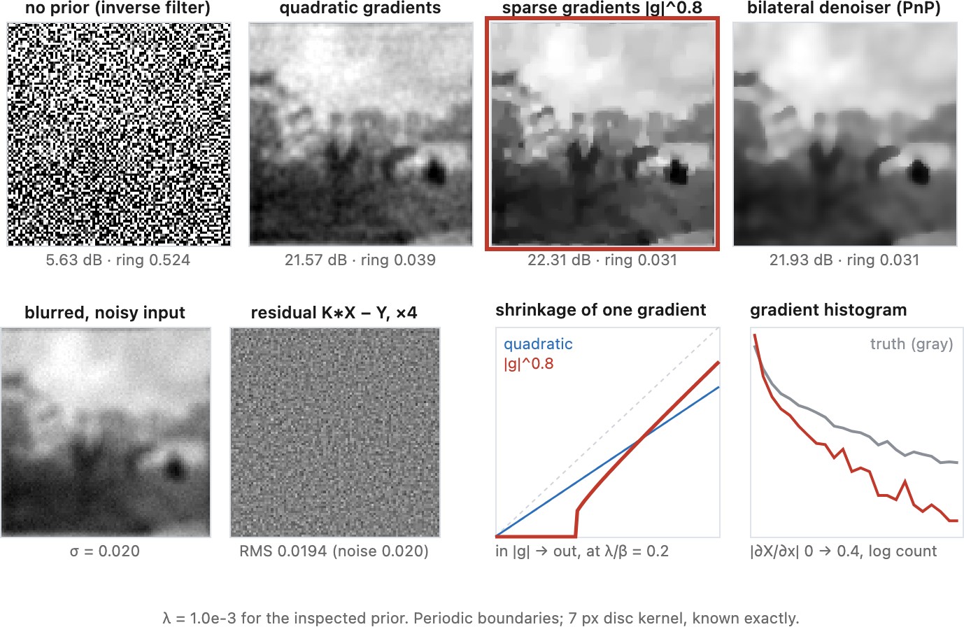
A power-spectrum model summarizes second-order image statistics. Sparse-gradient priors additionally favor many small differences and fewer large ones, a useful model for edges and relatively smooth regions. Real photographs also contain dense texture. Compare gradient distributions rather than treating every scene as piecewise constant (Figure 16.4.4).
A squared-gradient penalty rewards spreading a fixed contrast over more pixels. Absolute or sublinear penalties reduce that preference (Chapter 13.5, Total variation and optimization-based denoising). This explains one edge tradeoff; ringing also depends on the inverse response, boundary conditions and kernel mismatch, not only the prior.
The fix is to change the prior, keeping everything else, the known kernel $K$ and the same data-fit term. Instead of the frequency-domain divide, deblurring becomes an optimization,
For componentwise differences, $\rho(g)=|g|^\alpha$ gives a quadratic roughness penalty at $\alpha=2$, anisotropic total variation at $\alpha=1$, and a nonconvex hyper-Laplacian penalty for $0<\alpha<1$. Isotropic TV groups the two gradient components before taking their Euclidean norm. Quadratic regularization corresponds to a particular Gaussian precision model, not every possible Wiener spectrum. None of these choices guarantees exact edge placement or ringing-free output.
Compare two ways to cross a unit step: one difference of magnitude one, or ten consecutive differences of magnitude one tenth. A quadratic gradient penalty assigns costs one and one tenth respectively, so it favors spreading the transition. An absolute-gradient penalty assigns both cost one. A square-root penalty assigns costs one and about 3.16, favoring the concentrated transition in this simplified comparison. The data term and surrounding image still matter, but this calculation explains why changing the exponent changes edge behavior. It also shows why a nonconvex sparse-gradient penalty is not interchangeable with total variation.
16.3.2 Solving it, and the trick that made it fast⧉
Iteratively reweighted least squares uses stabilized weights proportional to $(g^2+\epsilon^2)^{\alpha/2-1}$, with $\epsilon>0$ preventing an infinite weight at zero (Levin et al. 2007). Spatially varying weights generally require an iterative linear solve; the system is not diagonalized by one FFT.
Half-quadratic splitting introduces a gradient copy $v$ (Geman & Yang 1995 (half-quadratic); Krishnan & Fergus 2009):
Here $D$ is the discrete gradient and $\beta>0$ the splitting penalty. The first step is quadratic; periodic shift-invariant operators permit a Fourier solve. The second is a scalar minimization for componentwise penalties. Some exponents admit specialized analytic or table-based solutions; compare candidate minima, including zero, rather than choosing an arbitrary polynomial root. A continuation schedule changes $\beta$ and must be stated.
These methods can improve edge reconstruction, but nonconvex optimization can depend on initialization and schedule. The kernel is assumed known here. Blind methods may use different intermediate priors to estimate the kernel before a final image reconstruction; they need not use exactly the same objective at both stages.
The splitting algorithm exposes the two operations that the compact equation hides:
initialize image estimate and auxiliary gradient field
for each chosen positive penalty value:
    repeat until the inner stopping criterion:
        image = solve quadratic data fit plus gradient-agreement term
        gradients = spatial_gradient(image)
        for each gradient component:
            auxiliary = minimize scalar sparse penalty
                        plus quadratic distance to that gradient
return image
The image update uses the forward operator and its boundary conditions. It can be diagonalized by FFT when the relevant operators are shift invariant with compatible periodic boundaries; spatially varying weights generally require a different solve. The auxiliary update is a scalar problem for a separable componentwise penalty. A vectorial or isotropic gradient penalty couples components instead. For nonconvex penalties, initialization, continuation, and selection among candidate scalar minima can affect the result.
The reweighting has a useful local interpretation. With a subquadratic gradient penalty, a small estimated gradient receives a relatively large quadratic weight and is pushed toward zero. A large gradient receives a smaller weight and can remain an edge. The next image estimate changes those gradients, so the weights must be recomputed. A positive stabilizer prevents the weight from diverging at zero; the iteration also needs a stopping rule. Half-quadratic splitting separates the work differently: the image update enforces the global blur model, while an auxiliary gradient update handles the nonquadratic penalty. This division explains why a difficult image prior can coexist with a comparatively simple global solve.