16.2 Non-blind deconvolution⧉
A known blur still leaves a difficult reconstruction when it suppresses signal below the noise. Wiener filtering Wiener 1949 uses second-order statistics, while Richardson–Lucy uses a Poisson likelihood. Their assumptions and stopping choices differ.
16.2.1 The Wiener filter: the regularized, noise-aware inverse⧉
The idea in one line: take the naive inverse filter and attenuate it wherever noise would dominate, frequency by frequency, with the amount of attenuation set by the signal-to-noise ratio at each frequency. Where the data is trustworthy, invert fully; where it is noise, hold back.
Written per frequency in the Fourier domain, the Wiener filter is
Here $H^*$ is the complex conjugate of the blur response, $S_x$ the latent-image power spectrum and $S_n$ the additive-noise power spectrum. The ratio $S_x/S_n$ is a power ratio before blur; the observed signal-to-noise ratio includes $|H|^2$. Where $S_x>0$, the filter is $H^*/(|H|^2+S_n/S_x)$.
For nonzero $H$ and vanishing $S_n/S_x$, the filter approaches $1/H$. For $H\to0$ and a positive noise-to-signal ratio, its response goes to zero. These are different limits; the noiseless zero-response case remains undetermined. Distinguish the reconstruction filter $F=H^*/(|H|^2+S_n/S_x)$ from its signal transfer $FH=|H|^2/(|H|^2+S_n/S_x)$. The latter lies between zero and one; the former can amplify measured values.
Wiener filtering minimizes mean squared error within the class of linear estimators using the specified means and covariances. Gaussianity is not required for this linear optimality. Joint Gaussian assumptions make the conditional mean linear as well. The Fourier form requires stationary statistics and compatible convolution boundaries; estimated spectra make it a plug-in approximation.
The regularizer modifies a normal-equation denominator, not the physical PSF. In a quadratic formulation, $(A^{\mathsf T}A+\lambda L^{\mathsf T}L)X=A^{\mathsf T}Y$ retains the measured operator $A$ and adds a penalty through $L$. Reinterpreting the resulting filter as an inverse of some response does not guarantee a nonnegative, normalized, physically realizable blur kernel.
Kernel accuracy and regularization interact, so evaluate sensitivity by perturbing the assumed kernel while keeping the solver and parameter-selection protocol controlled. A mismatch that happens to improve one result does not imply that the physically correct kernel should generally be replaced.
Figure 16.2.2 compares inverse and regularized reconstruction for selected kernels and noise levels. Sweep regularization to expose noise amplification and loss of detail; the measured scores depend on the image and settings.
A power-spectrum model does not capture all the local structure of edges and texture. Sparse-gradient penalties and learned denoiser priors offer other assumptions (Chapter 16.3, Priors for deconvolution, Chapter 13.11, Denoising as a universal prior). They can also introduce artifacts or fail under model mismatch.
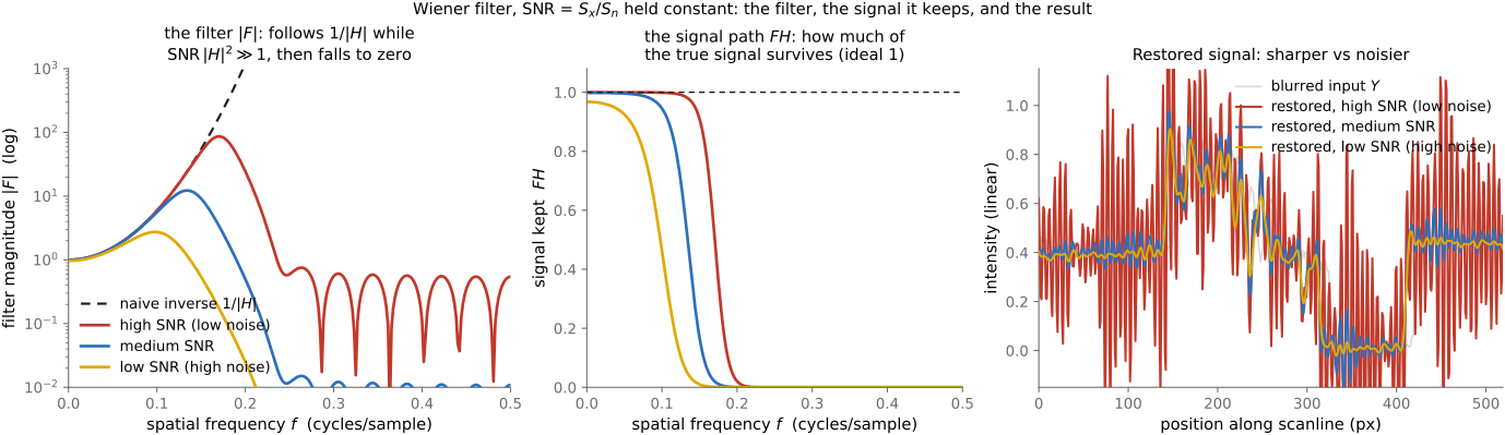
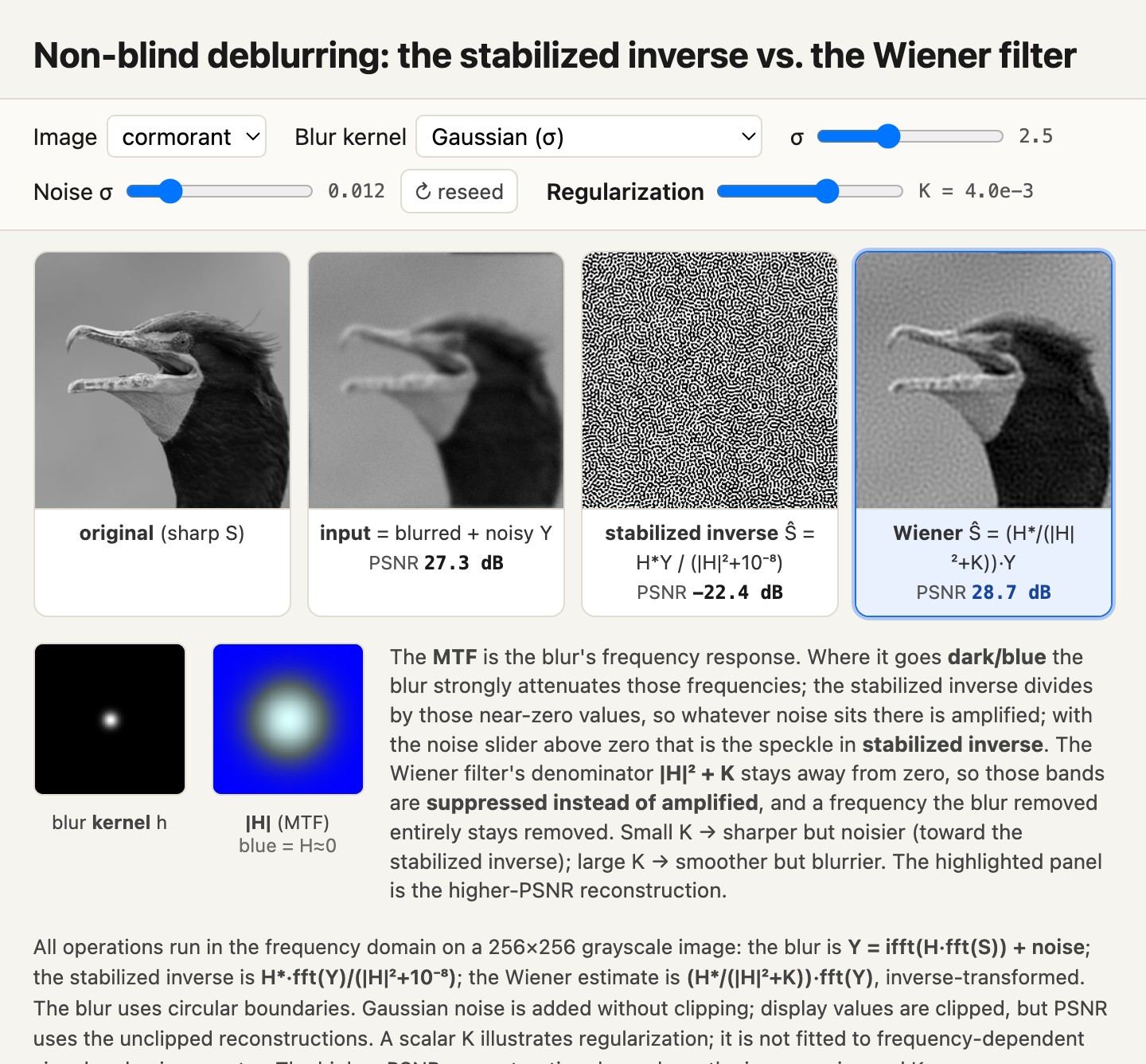
A frequency attenuated to one tenth of its original amplitude illustrates the danger of direct inversion: dividing by that transfer value multiplies measurement noise at the same frequency by ten. The Wiener estimate weighs that amplification against the expected signal power. When the observation contains little reliable evidence at the frequency, it accepts attenuation in the estimate rather than amplifying mostly noise. At a well-observed frequency, it approaches the inverse behavior. This is an estimator designed using the physical blur and the noise statistics; it need not be interpreted as the inverse of a different physically realizable point-spread function.
Kernel accuracy can be studied experimentally without confusing the blur model with the estimator. Hold the observation, noise model, boundary treatment, and reconstruction settings fixed. Perturb the estimated kernel's width, location, or trajectory, and inspect the change in the recovered image. A small kernel error near a poorly observed frequency can matter much more than a comparable error elsewhere. Then repeat at another noise level or regularization strength. This separates the sensitivity of the final reconstruction from the numerical distance between two kernels, and gives a more useful test than assuming that every improvement in kernel error must produce the same improvement in image quality.
The image spectrum is already a prior, even in this classical linear estimator. If the model expects little image power in a band, a measured fluctuation there receives less weight than the same fluctuation would under a model expecting strong signal. A power spectrum describes average energy by frequency, however; it does not tell us that several frequencies should align to form a particular sharp edge. That missing relationship motivates the sparse-gradient and richer image models in the next chapter.
16.2.2 Richardson-Lucy: iterate toward the likelihood⧉
Photon-counting applications motivate a Poisson likelihood. Read noise, background and detector calibration still matter; astronomy and microscopy do not universally have pure Poisson noise.
For independent counts $y_i\sim\operatorname{Poisson}((Ax)_i+b_i)$, with nonnegative operator $A$ and known nonnegative background $b$, minimize the Poisson negative log likelihood. Richardson–Lucy uses the update (Richardson 1972; Lucy 1974)
Products and divisions are pointwise. Predict the counts, compare observed to predicted counts as a ratio, back-project it through the adjoint, and normalize by sensitivity. The familiar formula without the denominator assumes $A^{\mathsf T}\mathbf1=\mathbf1$, which need not hold with cropping or boundary loss.
Three properties follow from that form and they are the reasons it survived.
It preserves nonnegativity when initialized nonnegatively with a nonnegative operator. Initialize supported unknowns positively: a zero component remains zero under multiplicative updates. Positive reconstructions can still ring or develop spurious peaks.
For zero background and a flux-preserving operator, the total estimate after an update equals the total observed counts. It does not generally preserve the initial estimate's flux, nor does this identity guarantee unbiased photometry in finite apertures. Cropping, background and regularization change the relation.
The ratio follows from the Poisson likelihood. Subtracted backgrounds can produce negative observations that do not fit that model. Use a suitable likelihood or preprocessing convention when read noise and offsets are significant.
Driving a weakly constrained likelihood too far can amplify noise. Early stopping regularizes the estimate; choose it using validation, a noise-aware discrepancy criterion or a declared budget. An explicit prior changes the optimization problem. A maximum-likelihood solution is not intrinsically pure noise, but can overfit the measured fluctuations.
sensitivity = A_adjoint(ones_like(y))
x = positive_initial_estimate()
for t in range(maximum_iterations):
    predicted = A(x) + background
    ratio = y / maximum(predicted, numerical_floor)
    correction = A_adjoint(ratio)
    x[sensitivity > 0] *= correction[sensitivity > 0] / sensitivity[sensitivity > 0]
# zero-sensitivity unknowns have no data support; mask or constrain them explicitly
16.2.3 Constraints instead of priors⧉
Van Cittert adds a scaled residual, $x^{t+1}=x^t+\eta(y-Ax^t)$, when data and unknown occupy the same space. Least-squares gradient descent instead uses $\eta A^{\mathsf T}(y-Ax^t)$, called a Landweber step. They coincide only in special cases. Convergence requires suitable operator and step conditions. Constrained least squares (Hunt 1973 (constrained least squares)) limits roughness or another property; under suitable convexity and constraint qualifications it relates to a penalized formulation.
A spectrum, an explicit penalty, a constraint and early stopping express different reconstruction choices. They should not be described as identical objectives merely because each can limit noise amplification.