7.5 Image priors🔗⧉

An image prior expresses which explanations of a measurement we favor. Smoothness, sparse gradients, patch statistics, and learned denoisers make different assumptions about photographs. The same prior can be used with several forward models, but its suitability still depends on the image domain and noise level.

Write the restoration objective as $\tfrac12\|Ax-y\|^2+\lambda\Phi(x)$. The data term measures agreement with the observation; $\Phi$ favors particular image structure. This unweighted data term assumes white noise, with its scale absorbed into $\lambda$. Correlated or signal-dependent noise requires the likelihood developed in Chapter 7.1, Imaging as Bayesian inference with probabilistic priors.

7.5.1 A catalog of priors: from smoothness to learned🔗⧉

A useful prior favors the structure one wants to preserve without assigning the same preference to noise or artifacts. No single assumption describes every part of every photograph.

A quadratic gradient penalty, $\Phi(x)=\|\nabla x\|^2$, penalizes rapid variation. It leads to a linear estimator with a quadratic data term, although the penalty itself is quadratic, not linear. By contrast, $\|x\|^2$ shrinks intensities toward zero without specifically favoring smoothness. Fourier diagonalization further requires compatible stationarity and boundary assumptions [@tikhonov-1963; @wiener-1949].

Wavelet sparsity assumes that much of an image can be represented with relatively few large transform coefficients Mallat 1989. The penalty $\|Wx\|_1$ sums coefficient magnitudes; counting nonzeros would be $\|Wx\|_0$. For pure denoising with an orthonormal $W$, minimizing $\tfrac12\|x-y\|^2+\lambda\|Wx\|_1$ gives

General inverse problems and redundant transforms need more than one thresholding pass. Large edge coefficients may survive, but weak detail can disappear and retained coefficients are biased toward zero Donoho & Johnstone 1994.

Sparse-gradient priors favor many small differences and fewer large ones. Isotropic total variation is

the anisotropic version sums $|(D_xx)_i|+|(D_yx)_i|$ Rudin, Osher & Fatemi 1992 (TV). TV can retain jumps but also flatten texture and create staircasing. Hyper-Laplacian penalties use powers below one, for example $\sum_j |(Dx)_j|^\alpha$ with $0<\alpha<1$ [@levin-etal-2007; @krishnan-fergus-2009]. The fitted exponent depends on the data and scale, and the objective is nonconvex.

In blind deblurring, jointly optimizing the image and blur under such priors can favor an incorrect nearly delta kernel. Levin and colleagues explain why marginalizing over possible images can improve kernel estimation Levin et al. 2009. This is not a universal inequality saying blur always reduces a sublinear gradient penalty: spreading one jump over many pixels can increase that penalty. Nor is marginalization the only successful kernel-estimation strategy; see Chapter 16.4, Blind deblurring.

Curvelets use elongated, oriented elements to represent edges efficiently Candès & Donoho 2004 (curvelets); shearlets provide another directional multiscale construction. These representations ask whether an edge can be described with fewer significant coefficients than in a less directional basis. The same preference for sparse coefficients appears in compressive sensing, although successful recovery additionally requires suitable measurements and assumptions. A sparse representation alone does not prove that an arbitrary camera can recover it.

7.5.2 The Gaussian prior in closed form: the Wiener filter🔗⧉

Assume a zero-mean stationary Gaussian image with power spectrum $S_x$, independent stationary Gaussian noise with spectrum $S_n$, and convolution by a known kernel $k$. On a periodic finite domain, or under the corresponding infinite-domain assumptions, Fourier coefficients decouple. The posterior mean and mode coincide, giving the Wiener estimate:

This is the Wiener filter Wiener 1949. In the quadratic solve of Chapter 6.9, Efficient linear solvers, the term $\lambda|\hat D|^2$ plays the role of $S_n/S_x$ when the chosen prior and noise model match. A gradient penalty corresponds to inverse power proportional to the squared derivative response; the continuous low-frequency form is $S_x\propto1/|\omega|^2$. Its unpenalized constant mode needs separate treatment, such as a specified image mean. An arbitrary regularizer is not automatically the correct Wiener model.

Approximate inversion requires the post-blur signal power $|\hat k|^2S_x$ to dominate $S_n$, not merely $S_x\gg S_n$. With positive noise power the gain tends to zero as $\hat k$ tends to zero. For pure denoising, $\hat k=1$, the estimate becomes $\hat x=S_x\hat y/(S_x+S_n)$. It shrinks each coefficient according to the assumed signal and noise powers.

A stationary linear filter applies the same frequency response everywhere. It cannot adapt separately to a smooth sky, a sharp silhouette, and fine foliage. Spatially adaptive priors can make those distinctions, at the cost of additional assumptions and computation. See Chapter 16.2, Non-blind deconvolution for the applied deblurring problem.

7.5.3 Shift and scale invariance🔗⧉

Translation and scale regularities make image models reusable, but both are approximations with limits.

Stationarity assumes that translating a feature does not change its probability. This is useful for local texture models; it is less appropriate for whole photographs with preferred layouts, such as sky above ground. Shared convolution weights provide translation equivariance of a mapping under compatible boundaries, not invariance of its output. Striding, padding, and positional inputs can break that equivariance.

Across a limited range of scales, ensembles of photographs often show an amplitude spectrum roughly proportional to $1/f$, corresponding to power roughly proportional to $1/f^2$ [@field-1987; @ruderman-1997]. This empirical tendency motivates multiscale models. It does not make photographs indistinguishable at every magnification: object sizes, optics, sampling, and noise introduce characteristic scales.

A prior may exploit these regularities locally while allowing position-dependent or scale-dependent behavior where the application needs it.

The dead-leaves model generates images by layering opaque random shapes [@lee-mumford-huang-2001; @ruderman-1997]. Suitable size distributions produce approximate scale regularities and image-like edge statistics. Occlusion alone does not guarantee a particular spectrum; the size law and its cutoffs matter. This is already a sampleable prior, without a neural network.

Fields of Experts learns filter-response potentials Roth & Black 2005 (Fields of Experts). K-SVD learns a sparsifying dictionary Aharon, Elad & Bruckstein 2006 (K-SVD). EPLL aggregates a learned patch log-likelihood over overlapping image patches Zoran & Weiss 2011 (EPLL). Trainable reaction–diffusion learns filters and nonlinearities in an iterative architecture Chen & Pock 2017 (TNRD); stage-dependent updates need not minimize one fixed energy. Learned penalties and learned update rules should be distinguished.

Two more specific assumptions are useful across several applications: local orientation and low-dimensional color variation.

The dead-leaves construction is useful because we can inspect which assumption creates which image property. Draw one opaque shape, then another over it: the newer shape hides part of the earlier one and creates an occlusion boundary. Repeating this at a range of sizes produces edges and regions without hand-drawing an edge map. Changing the size distribution changes the balance of broad regions and fine structure. Unlike a penalty that merely scores an input image, this construction supplies a procedure for drawing an image. The chosen shape, color, and size distributions determine how far its statistics resemble photographs.

A stationary local penalty often takes the form of a sum over positions of the same function of a neighborhood. Moving a texture then moves the terms without changing their form, apart from boundaries. Weight sharing in a convolutional network exploits a related reuse of local computation. A multiscale model extends that reuse across blur and sampling levels, while still allowing different noise scales and characteristic object sizes. These assumptions explain the mathematical forms of the models, not merely the appearance of their outputs.

The learned models also differ in what they fit. A Fields of Experts model learns both filters and the costs assigned to their responses. K-SVD learns atoms in an overcomplete dictionary so a patch can be approximated by a sparse combination. EPLL fits a Gaussian mixture to patches, then uses the sum of overlapping patch log-likelihoods as an image prior. Overlap couples the patch estimates into one image. A trainable reaction–diffusion model instead learns an iterative update procedure. These are intermediate steps between fixed hand-written penalties and a general learned denoiser.

7.5.4 Anisotropy: sparsity in a single direction🔗⧉

The sparse-gradient priors say an image is mostly flat. There is a stronger, more structured statement hiding inside many algorithms: where an image does vary, it tends to vary in one direction. Near an edge the intensity changes sharply across the edge and barely at all along it: locally, the image is essentially a one-dimensional signal embedded in two dimensions, its gradient field locally rank-one. This is anisotropy, and it is best read as a special, oriented form of sparsity: not merely "few non-zero gradients," but "the non-zero gradients all point the same way."

Near a straight edge, neighboring gradients are nearly parallel. A local structure tensor makes this test explicit:

One large eigenvalue and one small one indicate an edge with a well-defined normal; two small eigenvalues indicate a flat patch; two substantial eigenvalues indicate a corner or texture. Edge-directed demosaicking uses directional agreement to choose interpolation paths [@hamilton-adams-1997; @hirakawa-parks-2005]. It can fail where no single direction describes the neighborhood. Bilateral filtering also limits averaging across strong intensity changes, but does not require an explicit one-dimensional model in every window Perona & Malik 1990.

At a straight vertical boundary, neighboring pixels above and below a missing sample may remain on the same surface, while neighbors to the left and right cross the boundary. Interpolating vertically can therefore preserve the transition better than averaging all four directions. At a corner, a crossing of lines, or a finely woven fabric, there may be no single reliable direction. An edge-directed method must then combine evidence or fall back to a less confident estimate. This connects the useful local one-dimensional model to the places where its assumption breaks, rather than treating edge direction as something the algorithm always knows.

7.5.5 Linear color models🔗⧉

Colors in a small patch often occupy a low-dimensional subset of RGB space. A single material under varying scalar illumination traces a line through the origin; blends of two fixed colors trace an affine line. Two independently shaded materials can span a plane, so a color line is an assumption to check, not a consequence of having only two materials Omer & Werman 2004 (color lines).

For fixed foreground and background colors, matting uses $I=\alpha F+(1-\alpha)B$. If $F\ne B$, opacity is an affine function of color:

When $F=B$, color provides no opacity information. Closed-form matting extends local color assumptions to a quadratic cost in the unknown opacity field, eliminating local color coefficients to obtain a sparse matting Laplacian Levin, Lischinski & Weiss 2008 (closed-form matting). Foreground/background constraints and regularization resolve ambiguities. “Closed form” here still entails a global linear solve; the local prior alone does not determine a unique matte.

Plotting local pixels in RGB space exposes a kind of structure that a spatial smoothness penalty does not describe. A patch can change sharply in intensity while remaining close to a color line. Conversely, two nearby pixels can be spatially close but belong to unrelated materials. Local color models recur in matting, demosaicking and haze-related reasoning because they constrain which color changes are plausible. They must be checked against specular reflection, mixed illumination and multiple materials; these can expand the color distribution beyond the assumed line.

7.5.6 Denoising as a universal prior: Plug-and-Play and RED🔗⧉

A splitting method exposes a useful relationship between explicit regularizers and denoisers.

Half-quadratic splitting introduces a copy $v$ and minimizes

Alternation separates a data-fit solve from a prior update. The latter minimizes $\tfrac12\|v-z\|^2+(\lambda/\rho)\Phi(v)$, a Gaussian MAP denoising objective with effective variance $\sigma^2=\lambda/\rho$ when $\Phi$ is the negative log-prior. A fixed finite $\rho$ defines a penalized split problem; continuation toward large $\rho$ enforces agreement. ADMM uses an additional dual variable and different updates.

Plug-and-play replaces the proximal update with a denoiser $\mathcal D_\sigma$, which need not have a known penalty behind it Venkatakrishnan et al. 2013. An HQS-style iteration is:

v ← initial reconstruction
for each rho in the chosen continuation schedule:
    solve (AᵀA + rho I) z = Aᵀy + rho v
    sigma ← sqrt(lambda / rho)
    v ← D_sigma(z)
    check data residual and change in iterates
return v

The Gaussian variance interpretation is exact for the matching proximal model. For a trained denoiser it is a calibration convention whose intensity scale and noise parameter must agree with training.

The forward model enters the data solve, allowing reuse of a denoiser across tasks. Reuse still requires compatible intensity units, color space, noise levels, and image statistics. An arbitrary denoiser may not be a proximal operator, and the iteration may fail to converge. Better denoising benchmark scores do not guarantee better restoration in this loop. FlexISP illustrates joint camera processing with optimization and image priors Heide et al. 2014.

Regularization by Denoising (RED) proposes $\Phi(x)=\tfrac12x^\top(x-\mathcal D(x))$ Romano et al. 2017. Differentiating a differentiable denoiser gives

This reduces to $x-\mathcal D(x)$ when local homogeneity gives $J_{\mathcal D}(x)x=\mathcal D(x)$ and the Jacobian is symmetric. Common denoisers need not meet these conditions Reehorst & Schniter 2019 (regularization by denoising, clarified). Iterations using the residual can still be useful, but one cannot generally claim that they descend this explicit energy. PnP fixed points, RED residual equations, and MAP minimizers are distinct concepts.

This is also exactly the mechanism by which the not-optional prior of L7.8show (from Chapter 14.1, What can super-resolution actually do?) actually enters the computation: the denoise step is the prior step. It is also the concrete form of the learned-operator lesson L7.6show: when $\mathcal{D}$ is a learned denoiser, you have swapped a hand-designed prior for one learned from data, while the data-fit + prior skeleton stays put.

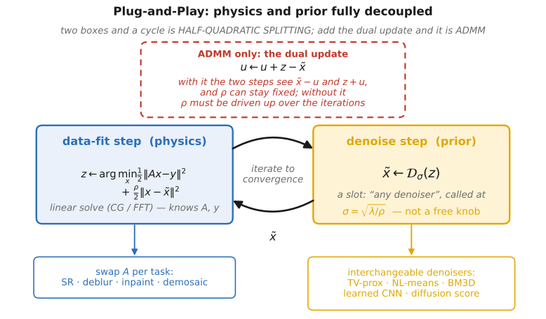
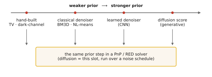
The split can be read directly from the two competing requirements. The data step asks for an image that explains the measurement while staying near the current denoised estimate. The denoising step asks for a nearby image favored by the chosen image model. For super-resolution, the data operator blurs and subsamples; for inpainting, it selects observed pixels. That operator can change while the denoiser interface stays the same. This reuse is the practical appeal of the construction, subject to the compatibility conditions above.

7.5.7 Denoisers and noise-dependent scores🔗⧉

An exact Gaussian MMSE denoiser determines the score of a noisy-image distribution. This identity explains a connection to diffusion without identifying restoration optimization with sampling.

Tweedie's formula. Suppose you observe a clean image corrupted by Gaussian noise, $z = x + \sigma\epsilon$. The best possible denoiser in the mean-squared sense, the minimum mean-squared error (MMSE) estimator, which is the posterior mean $\mathbb{E}[x \mid z]$, has a simple form:

Here $\epsilon\sim\mathcal N(0,I)$ is independent of $x$, and $p_\sigma$ is the Gaussian-smoothed image density. Its score points toward increasing noisy-image density. The identity gives the posterior mean, which need not lie on a clean-image manifold or equal a most probable image. A trained denoiser only approximates it.

Chapter 7.4, Generative AI and diffusion uses a family of scores at different noise levels to define a reverse sampling process [@ho-etal-2020; @song-etal-2021]. The schedule, drift, and stochastic or deterministic sampler determine its distributions. This is not the continuous limit of a generic PnP or RED optimization loop.

Conditioning such a process on measurements requires the posterior score at each noise level. Applying the clean-image forward model directly to a noisy diffusion state generally gives the wrong likelihood. Practical algorithms approximate that conditioning in different ways; the denoiser-to-score identity alone does not solve it.

For implementation, determine whether the network predicts a clean image, noise, a score, or a velocity. Conversion depends on the corruption parameterization. A plug-in name is not a sufficient interface specification.

7.5.8 Score-based models, the thin manifold, and imperfect priors🔗⧉

Noise smoothing helps define and learn scores, but it does not remove model error.

Natural images occupy a restricted, highly structured region of pixel space. An exact lower-dimensional distribution has no ordinary full-dimensional density; a density that is merely small can still have a well-defined score. Convolution with Gaussian noise gives a positive smooth density for every $\sigma>0$ Song & Ermon 2019. Training at multiple noise levels provides examples away from clean images. Neither positivity nor smoothing guarantees an accurate learned score everywhere, and a posterior-mean correction need not be an orthogonal projection onto a manifold.

A diffusion prior need not expose an easily evaluated clean-image density. Probability-flow methods can nevertheless estimate likelihoods, and a normalizing constant independent of the image is not needed for a score. The main conditioning difficulty is relating measurements of a clean image to intermediate noisy states. Approximate guidance and a mismatched prior can alter both residuals and uncertainty. Feng and colleagues study using score-based models as Bayesian imaging priors Feng et al. 2023. Evaluate measurement agreement and posterior behavior separately from visual plausibility.

How such a prior generalizes from finite data is itself an empirical question. Kadkhodaie, Guth, Simoncelli and Mallat trained denoisers on two non-overlapping sets of face images: with small sets each network memorized its own training images, but with large enough sets the two networks learned nearly the same score and generated nearly the same image from the same noise, which is generalization rather than recall Kadkhodaie, Guth et al. 2024. They trace this to an inductive bias of the networks toward what they call geometry-adaptive harmonic bases, oscillating patterns that follow the contours of the image. The finding is specific to the architectures and data they studied; it explains why a denoiser can serve as a prior beyond its training set, not that it always will.

Choose an explicit prior when its assumptions fit and its optimization is useful. Choose a denoiser or generative model when its learned image statistics justify the added complexity. In either case, validate the forward model, boundary handling, noise scale, and behavior on images outside the training distribution.