5.2 Exposure and capture timing⧉
A bright preview does not tell us whether the camera collected enough light. It may have amplified a short, noisy exposure. Choose integration time for motion and aperture for the required depth of field, then work out whether the scene supplies enough photons at those settings.
Optical exposure is light integrated at the sensor. Rendered brightness is a result of gain, development and display. Keeping these quantities separate prevents many mistakes with ISO and exposure compensation.
5.2.1 Basic photography: exposure settings (shutter, aperture, and ISO)⧉
For an unchanged scene and lens transmission, optical exposure scales as
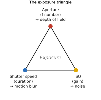
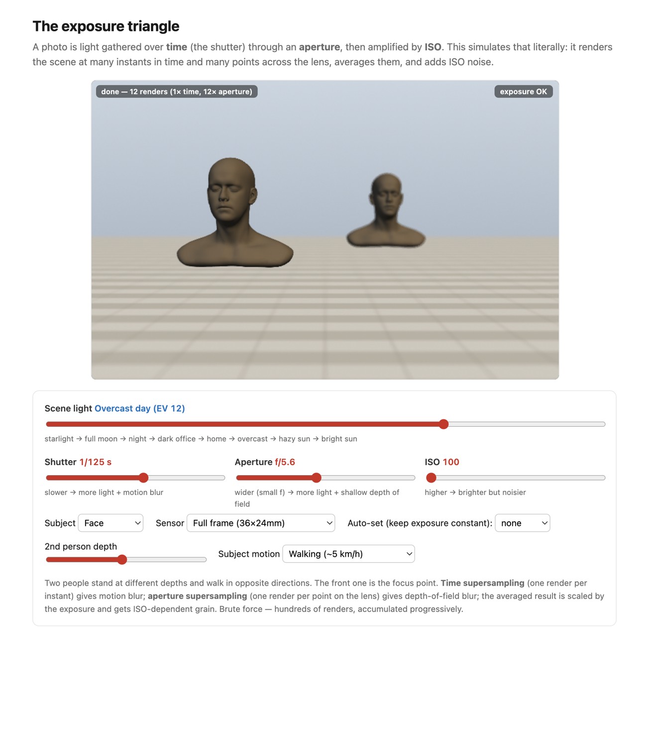
Twice the integration time collects twice the light. Multiplying the f-number by $\sqrt{2}$ halves it. Thus f/2.8 at 1/250 s and f/4 at 1/125 s give approximately the same optical exposure, but the longer integration blurs motion more and the smaller aperture increases depth of field.
A stop is the base-two logarithm of a light ratio. The setting-based exposure value uses time in seconds:
Increasing this EV by one halves optical exposure. Positive exposure compensation is a different convention: it asks an automatic mode for a brighter result relative to its metered choice. In aperture priority at fixed ISO, +1 stop will ordinarily double time. In manual mode with Auto ISO it may instead double gain while leaving the light collected unchanged.
ISO is not a third optical control. At fixed aperture and time, increasing gain scales the signal and its shot noise together. It can reduce the importance of noise added downstream of that gain, or select a sensor conversion-gain mode with lower input-referred read noise. It can also reduce highlight headroom. On an ISO-invariant sensor over the relevant range, low-ISO raw data brightened later can be close to a higher-ISO capture. The comparison in Chapter 2.8, Noise, signal-to-noise ratio and dynamic range applies only after matching output brightness and checking clipping.
The common association between high ISO and noise usually includes a reduction in collected light: we raise ISO because the scene is dim or the shutter must be fast. Add light, open the aperture or lengthen time when the photograph permits it. Raising ISO alone does not improve photon statistics.
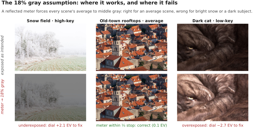
Reflected-light metering measures light coming from the scene; it cannot separate a dark object in strong light from a pale object in weak light without additional information. Spot metering makes the chosen patch explicit. Evaluative metering uses more of the frame and may use recognized subjects. A gray card is a useful reference under the subject's illumination, not proof that a meter assumes exactly 18% reflectance. Snow and dark clothing are good tests of when compensation is needed.
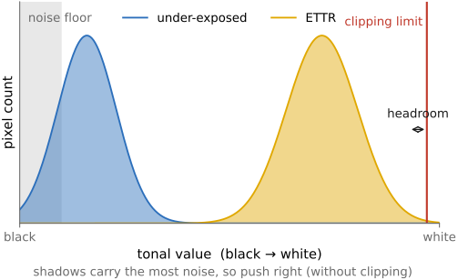
Expose to the right means collecting more light while retaining the highlights that matter. It is useful when time, aperture and saturation allow it; it is not a requirement to force every histogram against the edge. A longer exposure that blurs the subject is a poor trade for cleaner shadows. Inspect individual channels when possible, because a colored light can saturate one channel before the luminance preview looks white. Keep a margin when the camera's warnings refer to a processed preview rather than raw data.
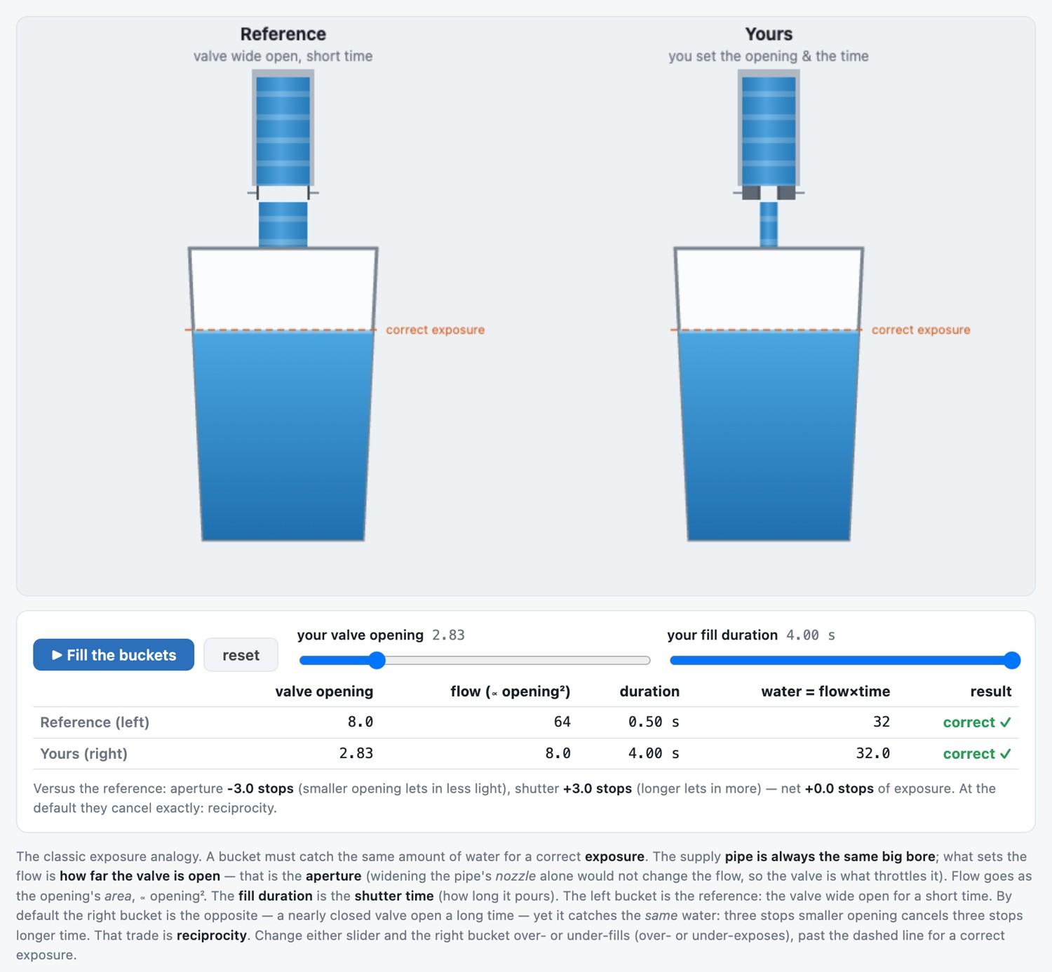
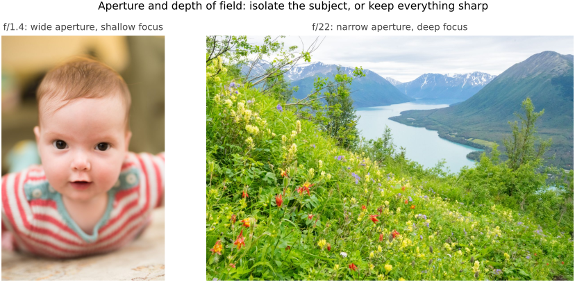
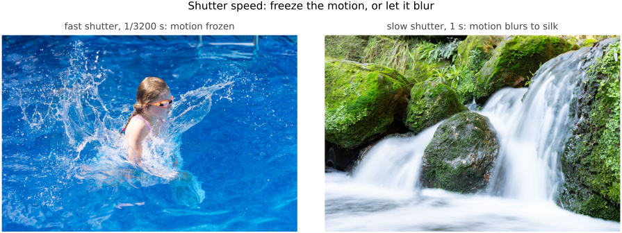
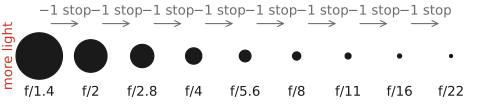
A stop is a factor of two. Time steps by two and f-number by $\sqrt{2}$. ISO and a software exposure slider can change rendered brightness by a stop without collecting another photon.
The f-number normalizes the physical opening by focal length. At the same f-number, a longer lens has a proportionally larger entrance pupil. For an extended scene of equal radiance, that compensates for the change in image scale so the on-axis irradiance is approximately unchanged, apart from transmission and close-focus effects. Aperture diameter alone would not give that useful comparison across focal lengths.
The familiar series f/1.4, f/2, f/2.8, f/4, f/5.6, f/8, f/11, f/16 follows from area. Each full-stop step multiplies the f-number by about the square root of two and therefore halves optical exposure at fixed time. Doubling time compensates for that step. For example, f/4 at 1/250 s and f/5.6 at 1/125 s collect approximately the same light per sensor area, with different motion blur and depth of field. Equal collected light does not make them interchangeable photographs.
5.2.2 Exposure modes, UI, and auto-ISO⧉
With fixed ISO, aperture priority selects time, shutter priority selects aperture, and program selects both. Manual fixes both and leaves the meter as advice. Each automatic mode has limits. Watch the selected values: aperture priority can choose a time too long for a moving subject, and shutter priority can run out of aperture in a dim room.
Auto ISO adds a variable. Manual with Auto ISO is useful when both motion blur and depth of field must stay fixed. Set a maximum ISO and know what the camera does on reaching it. Aperture priority with Auto ISO may permit a minimum shutter time, but that minimum can be conditional and the camera may violate it when the gain limit is reached. A focal-length-based minimum addresses camera shake; it does not know how fast the subject moves.
For a person moving indoors, begin with a time short enough to retain the expression, choose an aperture that holds the required facial features, and let ISO follow the light. Make a test frame and inspect it. If detail is blurred, shorten time or add light; if the wrong eye is sharp, change focus; if highlights clip, revisit metering or the intended rendering. These are different failures, and one brightness slider cannot diagnose them.
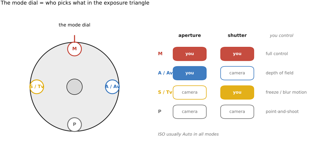
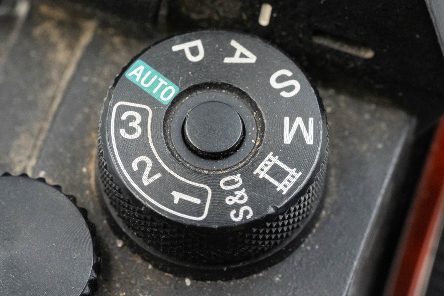
The names on the dial describe that division of responsibility:
| Mode | Photographer sets, with fixed ISO | Camera sets |
|---|---|---|
| P, program | A program choice or shift where available | Aperture and time |
| A or Av | Aperture | Time |
| S or Tv | Time | Aperture |
| M, manual | Aperture and time | Neither |
Program shift, when available, selects another aperture/time pair with approximately the same metered exposure. Scene modes add a guess about the intended photograph, such as preferring a shorter time for sport. Auto ISO changes the table by allowing gain to vary too. Exposure compensation biases an automatic choice; inspect which variable actually moved before assuming the camera collected more light.
5.2.3 Metering: from printed guides to the sensor⧉
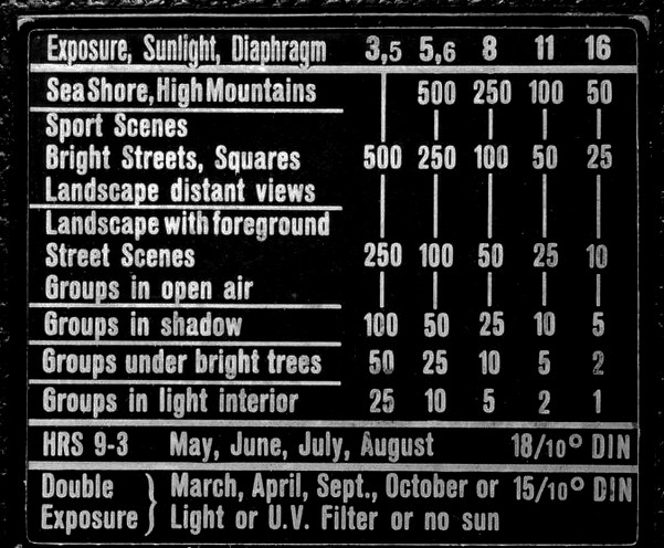
Before built-in meters, exposure tables related film speed to illumination and subject conditions. A handheld incident meter measures light arriving at the subject, while a reflected meter measures light leaving a selected area. Through-the-lens metering accounts for some effects of the actual optical path. None of these devices knows which part of a photograph we intend to emphasize.
For repeatable work, meter a defined patch or use a controlled reference under the same illumination. Record compensation and whether settings were locked. Absolute photometry requires more than the settings printed in EXIF; Chapter 17.2, Camera response and radiance calibration develops that distinction.
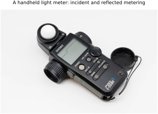
A reflected reading changes when a gray card is replaced by a white card under the same light. If an automatic system treats the brighter reading as a reason to shorten exposure, it can render the white card too dark. An incident reading taken at the subject responds to the illumination instead of that change of card reflectance. The white card can then remain lighter than the gray one under the same exposure. This is the practical attraction of an incident meter in a controlled setup; it does not determine the photographer's desired rendering.
The cost is access. You can aim a reflected-light spot meter at a distant subject from the camera position. Taking an incident reading requires sampling the light at a representative subject position and choosing how to orient the receptor. Mixed lighting and directional sources make that choice consequential. Meter type changes which quantity is measured, not whether judgment is needed (Figure 5.2.12).
Printed exposure guides made the first choice without measuring the scene. Film packaging and exposure calculators listed settings for bright sun, overcast light, and shade. The sunny-16 rule summarizes one such starting point: in bright sun, use f/16 and a time near the reciprocal of the film-speed number, about 1/100 s for ISO 100. It is a lighting estimate, not a measurement of every subject or a guarantee against clipped highlights.
Photocells made the estimate responsive to actual light. A separate or body-mounted meter could still see a different field from the taking lens and miss the loss from an added filter. Through-the-lens metering brought the measurement into the optical path that forms the photograph, accounting for transmitted light. Sensor-based metering brings it closer still: the camera analyzes a live readout from the imaging sensor. Preview processing and capture settings can differ, but the remaining decision, which tones matter and where to place them, still requires an inference about the scene and the photographer's intent.
5.2.4 f-stops versus T-stops⧉
Two lenses at f/2.8 need not transmit the same amount of light. The geometric f-number describes the entrance pupil. A T-stop includes transmission $\tau$:
A lens at f/2 with transmission 0.81 is approximately T/2.22. Its geometrical depth of field still depends on f/2. Through-the-lens metering can compensate for transmission loss in an automatic exposure; calibrated T-stop markings are useful when matching shots across lenses. Corner falloff and close-focus exposure changes require additional corrections, so a single T-stop is not a per-pixel radiometric calibration.
A transmission rating describes the lens under a specified measurement, but illumination can still vary across the frame. Oblique rays may see a smaller effective opening, and lens elements or the barrel can clip part of their bundle. In simple models the geometric falloff follows a cosine-fourth law; real wide-angle lens designs can depart from that model. Mechanical clipping often decreases when the aperture is stopped down.
A lens-shading correction multiplies darker corner values to make a uniform scene look more uniform. It multiplies their noise too. For example, a factor-of-two corner correction restores the mean brightness but also doubles the measured noise standard deviation at that location. It cannot replace the photons that the corner failed to collect. Exposure, vignetting correction, and visible corner noise should therefore be evaluated together.
Consider cutting between shots made with a prime and a zoom, with lighting and shutter time fixed. Equal f-numbers need not give equal recorded brightness if the two lenses transmit different fractions of the incident light. Through-the-lens automatic metering can compensate by changing another setting, but a manually controlled cinema setup needs a repeatable mark on the lens itself. T-stop calibration supplies that transmission-aware mark. The f-number remains the relevant geometric quantity for the ray cone and depth of field; matching exposure does not make two lenses optically identical.
5.2.5 Video capture settings⧉
For video, choose frame rate for the intended playback and motion sampling, then choose integration time for blur. Shutter angle $\theta$ expresses time as a fraction of one frame interval at rate $r$:
At 24 frames/s, 180° means 1/48 s. It is a familiar motion-rendering convention, not a physical definition of natural motion. A shorter integration gives sharper individual frames but can make movement look more staccato. Capturing at 120 frames/s and playing at 24 gives fivefold slow motion if each captured frame is used once.
A short integration does not necessarily shorten the time between the first and last row of a rolling-shutter frame. Check readout behavior for fast pans and moving subjects. Under flickering light, make a test clip: mains frequency alone does not describe every LED driver. Exposure time, readout timing and illumination can interact to produce bands.
Lock exposure and white balance when their automatic changes would be distracting within a shot, but allow tracking focus when subject distance changes. Log encoding allocates code values differently; it does not recover clipped sensor data. Record the profile and use its intended input transform when grading. Codec, bit depth and bitrate affect how much editing the file tolerates. The sampling and reconstruction consequences belong to Chapter 30.1, Motion blur, temporal sampling, and resampling and Chapter 30.2, Video compression and motion compensation.
5.2.6 Choosing one frame or several⧉
A burst can improve the chance of a useful expression without combining any frames. A denoising burst combines repeated measurements. Exposure bracketing varies time to retain bright and dark regions. These modes solve different problems.
Several frames help when corresponding scene points can be aligned and remain consistent. Moving hands, changing reflections and occlusions can violate that assumption even when the camera is held still. A longer total capture may also miss the intended instant. Keep a usable reference frame for important motion, and judge the merged result around moving boundaries as well as flat shadows. Stacking cannot restore an event absent from every input.
Recap: big lessons of this chapter
A stop is a factor of two. Time steps by two and f-number by $\sqrt{2}$. ISO and a software exposure slider can change rendered brightness by a stop without collecting another photon.