29.5 Scaling up Halide⧉
Larger pipelines add three complications to the blur in Chapter 29.4, Halide programming: reductions with constrained iteration order, producers shared by several consumers, and stages at different resolutions. The examples below isolate those problems. The interactive lab can help inspect them, but each scheduling decision should also be understandable from the dependencies and generated loops.
29.5.1 Decoupling storage from computation: store_at⧉
For the centered three-tap vertical blur, adjacent output rows need two horizontal rows in common. Computing a fresh three-row producer region for each output row repeats that overlap. Retaining the storage across rows permits reuse.
Follow three consecutive output rows. Output row 10 needs horizontal rows 9, 10, and 11. Row 11 needs 10, 11, and 12. Row 12 needs 11, 12, and 13. If we allocate a fresh intermediate for each output row, we produce nine horizontal rows for these three outputs, even though there are only five distinct rows in the union. The overlap is useful only if the values survive until their next use.
Allocation lifetime and computation placement therefore need separate controls. compute_at places the production of values inside a consumer loop. store_at, or store_root, can place their allocation outside that loop, so it survives successive iterations. Retaining an allocation makes reuse possible; the compiler must still recognize which values remain valid and which new values are required. This is why looking only at the location of an allocate statement does not establish how much arithmetic will run.
On a fresh copy of the float blur, keep the output's y traversal serial and use:
blur_x.store_root().compute_at(blur_y, y);
The allocation outlives each consumer row. When Halide recognizes the sliding-window pattern, it computes the initial needed rows, then only the newly required row, and can fold storage into a circular buffer. Inspect the lowered code to confirm the optimization and allocation size. store_root does not universally imply a small rolling buffer; that depends on accesses and schedule legality.
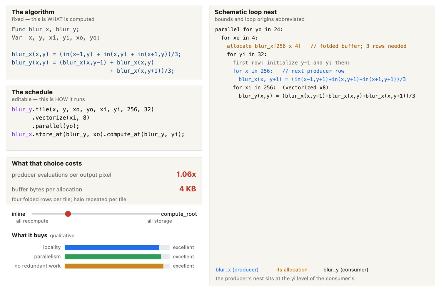
compute_at alone fixes both at once, compute a tile and store a tile, which is why computing per row on its own is the worst of both, a full recompute and a live buffer. Lift the storage to a coarser loop than the computation and the buffer outlives each chunk, so rows computed for one iteration are still there for the next: the sliding window. The loop nest splits in two when you do it, the allocate climbing to the outer level while the producer's loops stay deep inside, now computing only the one new row each output row needs, with Halide sizing the buffer from the stencil rather than from the chunk (for this 3-tap stencil it folds the storage to four rows). store_root() buys that at the price of serialising $y$; store_at(blur_y, yo) keeps the rolling window inside each strip (in a tiled schedule the equivalent is store_at the tile's $x$ loop, with the per-row compute at $y_i$), so the reuse survives and the strips stay independent, the one schedule cheap on all three axes at once.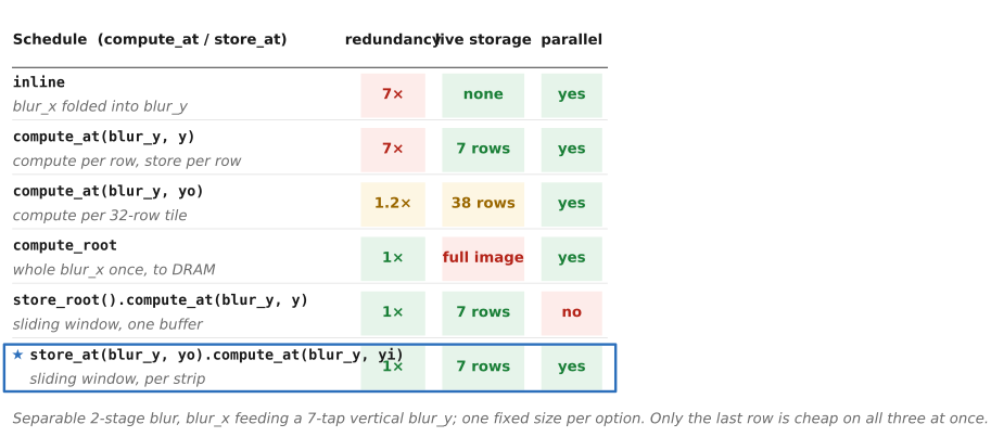
compute_at/store_at choice for the two-stage blur, one fixed size each, and what each pays on the three axes that fight. inline recomputes blur_x at every use (7× for a 7-tap vertical blur_y) but stores nothing; compute_at(blur_y, y) on its own is the worst of both, full recompute and a live buffer, the case store_at exists to fix; compute_at at the tile trades a small halo recompute for cache locality; compute_root removes all recompute but materializes the whole intermediate. Only the sliding window, storage lifted coarser than computation with store_at, computes each row once, keeps a handful of rows live, and, taken per strip, still runs in parallel: the one row cheap on all three at once.The sliding-window execution for this stencil can be read as follows:
allocate storage for three horizontal rows
produce horizontal rows -1, 0, 1 using the chosen input boundary rule
for output row y from 0 through H-1:
    compute output row y from retained horizontal rows y-1, y, y+1
    if another output row remains:
        replace the oldest retained row with horizontal row y+2
Three logical rows are live at a time. After computing output row 0, horizontal row -1 is no longer needed and its slot can hold row 2. The physical slot is reused while the logical row coordinate advances. This is storage folding, commonly implemented as a circular buffer. The compiler may choose a different physical allocation size, for example to simplify indexing, so the listing describes the required live values rather than a promised byte count.
For an output of height H, this traversal needs H + 2 horizontal rows including its halo, instead of producing three rows afresh for each of H outputs. Full materialization has the same set of required producer values, but keeps a much larger intermediate. The sliding window combines that reuse with a short lifetime for each value. Hardware image signal processors use the same line-buffer idea to process a stream without retaining every intermediate frame.
To recover parallel work, use independent strips, each with its own retained storage:
Var yo("yo"), yi("yi");
blur_y.split(y, yo, yi, 32, TailStrategy::GuardWithIf).parallel(yo);
blur_x.store_at(blur_y, yo).compute_at(blur_y, yi);
Rows within a strip advance serially; strips can run concurrently. The overlap is still recomputed at strip boundaries. For full strips with a radius-one vertical stencil, the geometric overhead is two extra producer rows per 32 output rows. Choose strip height from reuse, cache capacity, vectorization, and the number of available tasks. A shared rolling buffer cannot simply be reused by independently advancing workers.
For two adjacent strips, the retained values of one worker are unavailable to the other. A strip producing rows 0 through 31 needs horizontal rows -1 through 32; the next strip, producing 32 through 63, needs rows 31 through 64. Rows 31 and 32 are computed in both tasks. That small duplication makes the tasks independent. Taller strips reduce the duplicated fraction but expose fewer tasks and keep longer traversals on each worker. A useful schedule balances these costs rather than maximizing reuse at any price.
29.5.2 A 7×7 box blur: reductions and update definitions⧉
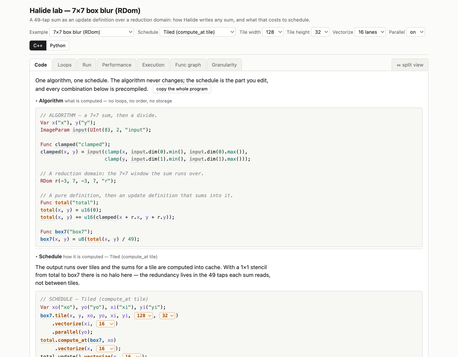
The direct box blur in Chapter 29.4, Halide programming initializes an accumulator, adds 49 input samples, and divides by 49. It has both a pure stage and an update stage, each with scheduling choices.
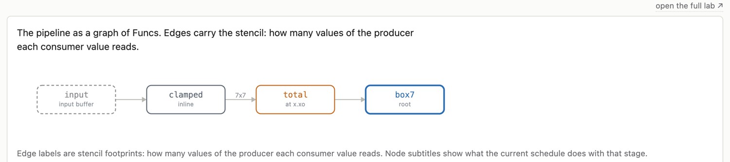
total, which accumulates 49 values per output pixel, and total feeds the divide. The 7×7 label on the middle edge is the stencil footprint, the number of producer values each consumer value reads.For a materialized total, vectorizing the pure initialization alone leaves the 49-tap update scalar. A schedule can also vectorize independent output coordinates in total.update(), while respecting the reduction variables' dependencies. Inspect the update loop order before choosing a vectorized dimension. Compare this direct algorithm with two separable seven-tap reductions when the goal is an efficient box blur.
A histogram instead scatters into shared bins. A safe parallel strategy gives each task a private histogram and combines them:
parallel for each image strip t:
    partial[t, 0:256] = 0
    for each pixel p in strip t:
        partial[t, input[p]] += 1
for each bin b:
    histogram[b] = sum over strips t of partial[t,b]
The temporary storage scales with strip count times bin count. Halide's rfactor can express suitable associative factorizations; it is not permission to parallelize an arbitrary update. A prefix scan, such as a histogram CDF, remains ordered unless rewritten as a parallel scan algorithm. Its initialization must include bin zero and its final result must include bin 255.
29.5.3 Harris corner detection: ten stages, fifteen edges⧉
Harris detection forms image gradients, smooths their products, and computes a corner response. With a local averaging operator $G$, the structure tensor and response are
A positive, sufficiently large response indicates variation in both directions for the chosen sensitivity $\kappa$. Thresholding and nonmaximum suppression are additional steps if the output should be discrete keypoints; see Chapter 12.3, Sparse matching. Here the response pipeline is useful because gradients feed several products and local sums.
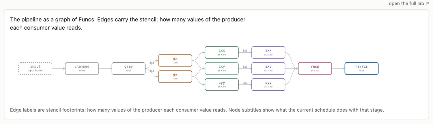
gray, the windowed sums read 3×3 of their products, and gray and the gradients each feed two consumers, which is exactly where storing once instead of recomputing pays. Node subtitles show what the current schedule does with each stage.Inlining can repeat shared producers; materializing every stage can create many full-image intermediates. Compare selective materialization with tile-local production. A cheap grayscale conversion is not automatically worth storing at root simply because several stages use it. Its cost must be weighed against the storage and traffic. Stencil halos compound backward through the graph, so a small output tile can require a much larger input region.
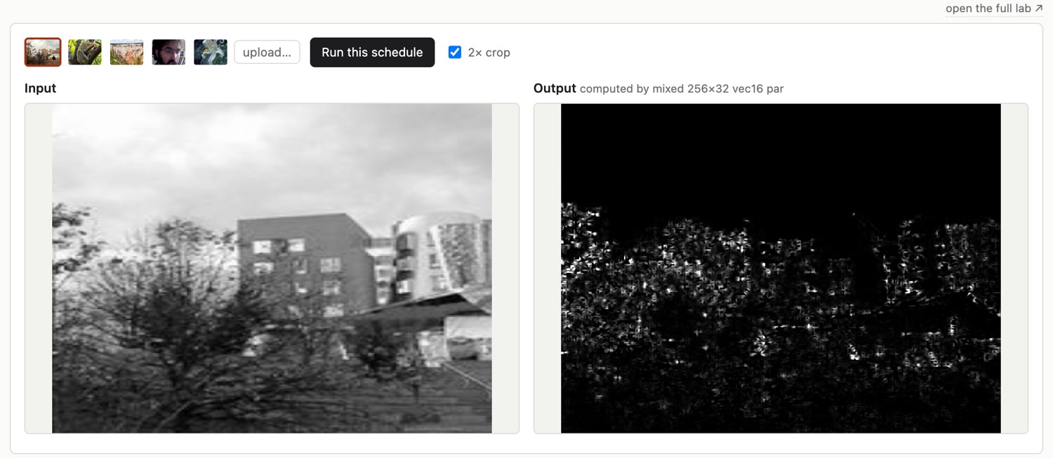
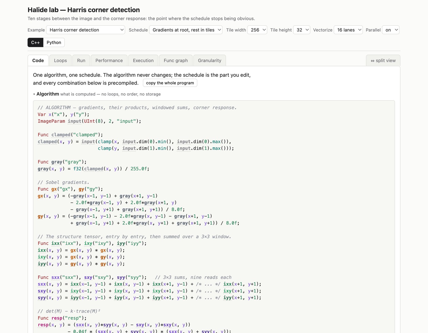
A shared grayscale producer makes the alternatives concrete. Inlining it into each derivative and neighborhood computation can repeat a small conversion many times. Storing a full grayscale image removes that repetition but adds writes, reads, and a buffer. Producing it within a tile limits the buffer while repeating work in overlapping halos. Which is cheaper depends on the conversion cost, the downstream stencil widths, and the memory hierarchy. The graph tells you where reuse exists; it does not by itself tell you where that reuse is worth materializing.
The corner criterion has a geometric motivation. A flat patch provides little evidence about either translation coordinate. Along a straight edge, displacement parallel to the edge changes the patch little. A corner contains variation in both directions, making its location more constrained. The structure tensor summarizes that directional variation; the response, threshold, and suppression turn it into a usable feature detector. Here those steps also provide a compact example of a graph with shared producers.
29.5.4 A brute-force bilateral filter: what a schedule cannot fix⧉
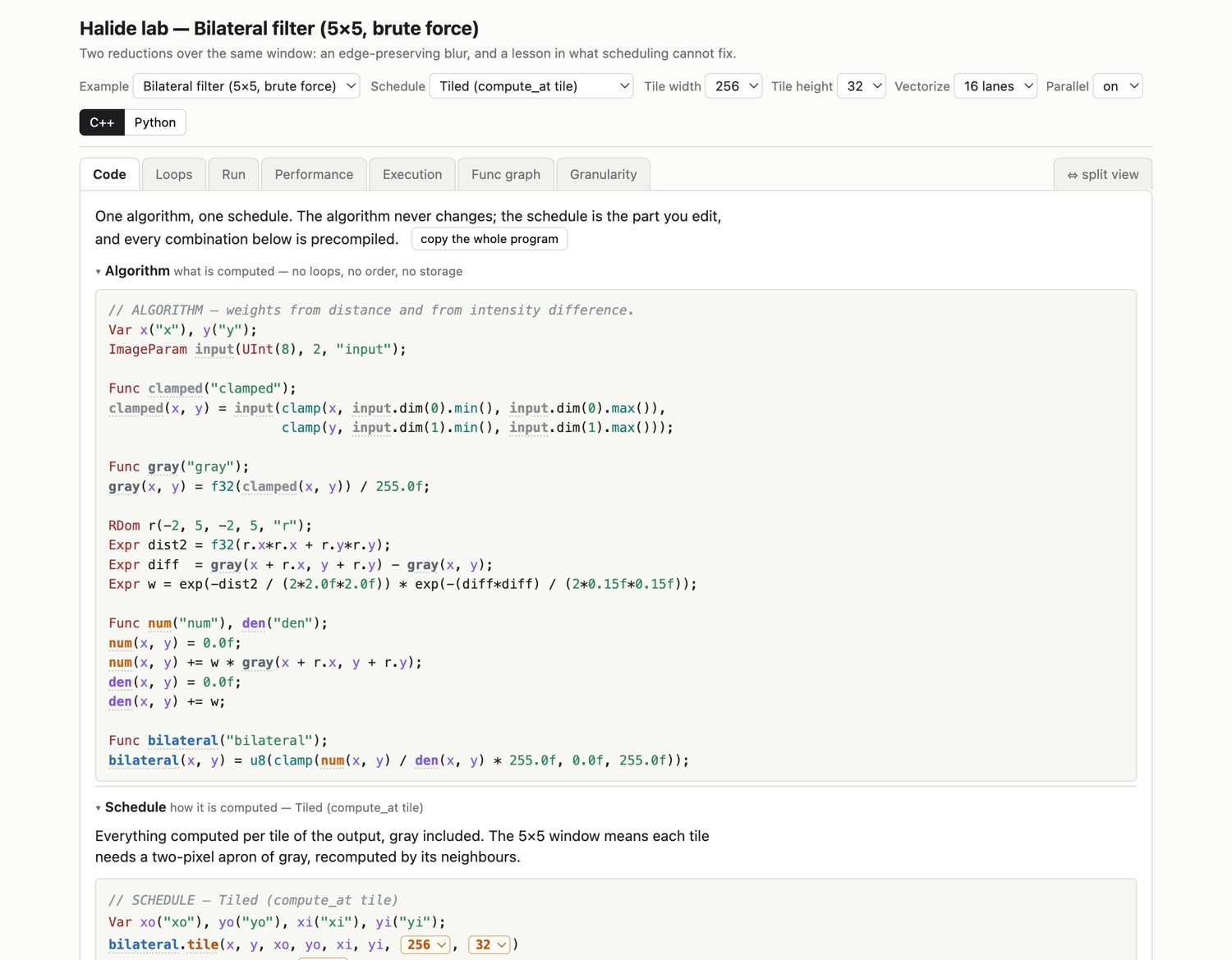
The bilateral filter accumulates weighted values and weights over a neighborhood, then divides. Range weights reduce the influence of neighbors whose intensities differ from the center. They do not categorically prevent mixing across every edge; see Chapter 10.1, Bilateral filtering.
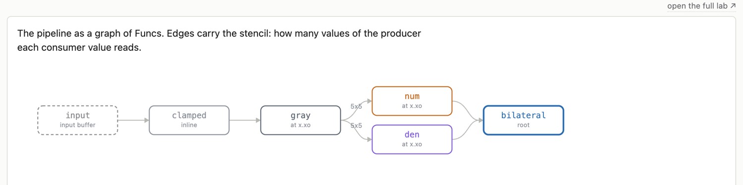
gray feeds both num and den with a 5×5 footprint, and the two meet again at the divide. That diamond is the structure worth staring at, because the two branches evaluate the same 25 weights independently.A tuple-valued accumulator can express both sums together. In pseudocode:
(value_sum, weight_sum) = (0, 0)
for each neighbor q:
    w = spatial_weight(p,q) * range_weight(input[p],input[q])
    (value_sum, weight_sum) += (w * input[q], w)
output[p] = value_sum / weight_sum
With positive bandwidth parameters and the center sample included, its weight keeps the denominator positive for finite inputs. Define a policy for nonfinite data and unsupported parameter values. A tuple exposes shared work, but separate expressions do not prove the compiler evaluates a weight twice; inspect lowered code.
29.5.5 The bilateral grid: changing the algorithm instead⧉
A bilateral grid Chen et al. 2007 splats values and weights onto a coarse spatial-intensity lattice, filters both, slices them at the output coordinates, and normalizes. The grid filtering is linear; the image-dependent splat and slice make the complete operation nonlinear.
If each spatial axis is reduced by eight and there are ten intensity bins, the grid has roughly $10/64$ as many cells as image pixels, before padding. Storing both values and weights gives about $20/64$ as many scalar entries. This is useful compression of the working set, but not “under 1%.” Spatial and range resolution, padding, and channel count all matter.
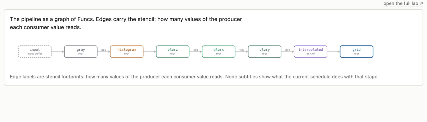
gray splats into histogram, the 3-D grid; three blurs run along the grid's z, x and y axes; interpolated slices the blurred grid back at full resolution, and the output divides value by weight. The scale factor of 8 on the splat and slice edges is the spatial downsampling, and gray feeding both the splat and the slice is the diamond that makes the grid work.Splatting is a scatter, so parallel updates need collision handling. Materializing a small filtered grid can be inexpensive; the full-resolution slice may then fuse with later point operations. A channel dimension of size two or a tuple can represent the value/weight pair, with different layout and scheduling implications.
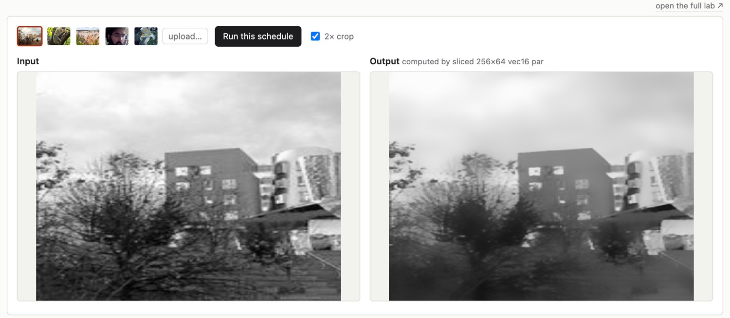
A wider direct filter costs more neighborhood work. A coarser spatial grid can keep its lattice filtering inexpensive, but splatting and slicing still visit every image pixel. Compare quality and speed at a matched target; a 5×5 direct filter and a much broader grid filter do not compute the same result.
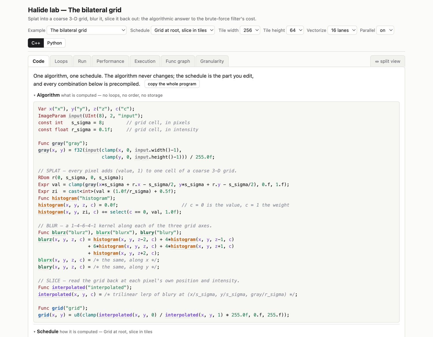
The splat, blur, and slice have different scheduling problems. During splatting, two distant input pixels can select the same coarse cell, so independent pixel work can collide at the output. During grid filtering, accesses are regular and the working set is much smaller. During slicing, the pipeline returns to full image resolution and interpolates values from the grid. Treating the three stages as if they had the same parallelism and storage needs misses the reason the representation is fast. Retaining a small grid can be inexpensive even when retaining a full-resolution intermediate is costly.
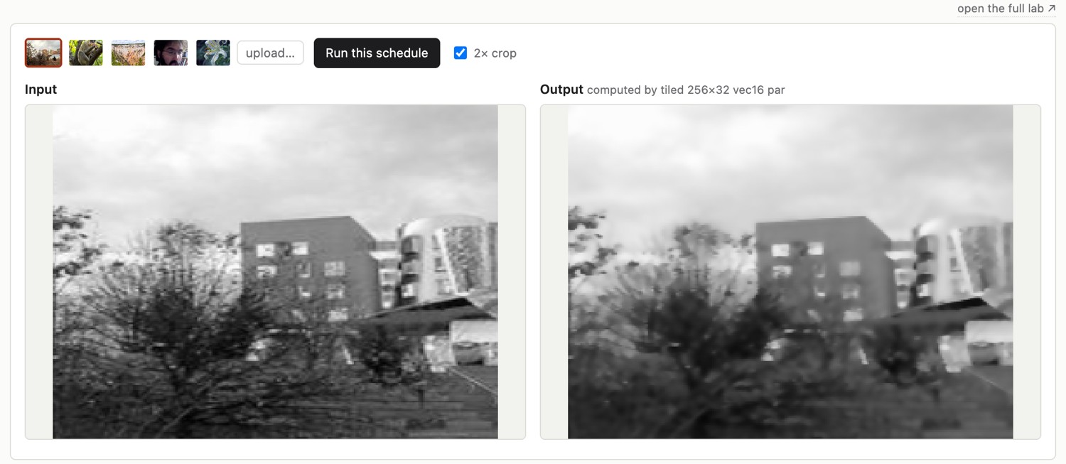
The timings show what the representation buys. Measured in the book's Halide lab on a 1024×768 image, single threaded on the author's laptop, the brute-force 5×5 bilateral filter took 35.6 ms with its best schedule (145 ms with a scalar root schedule), while the grid took 5.15 ms and filtered over a considerably wider window. The two do not compute the same filter, so this compares each method at a typical setting rather than two implementations of one filter. The gap widens with the filter width, because the grid's cost barely moves while the brute force grows with the square of the window. Scheduling moves work around; a better algorithm removes it. Both matter, and they are not substitutes.
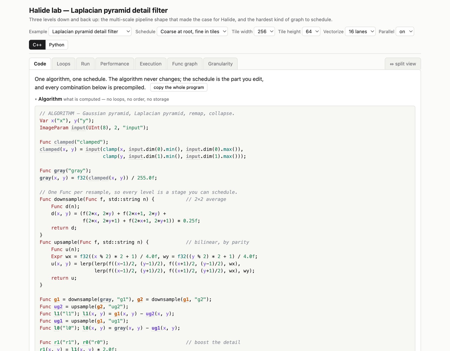
29.5.6 A three-level Laplacian pyramid: multi-resolution stages⧉
A Gaussian pyramid repeatedly low-pass filters and downsamples. A Laplacian band is the fine level minus an expansion of the next coarser level. Reconstruction adds the band to that same expansion, so the unmodified pyramid reconstructs algebraically, apart from finite-precision differences.
Multiplying detail bands changes local contrast and can produce halos or overshoot. It is a simple multiscale enhancement, not the full local Laplacian algorithm of Chapter 10.4, Local Laplacian filters, which uses intensity-dependent remapping. Chapter 6.6, Pyramids and wavelets defines the sampling conventions.
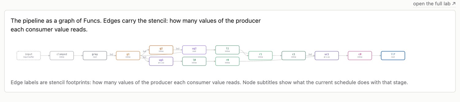
A fine output tile requests smaller coarse-level regions, each with its own halo. Recomputing coarse work per fine tile can become wasteful. Try materializing small coarse levels while fusing suitable fine stages. Deep inlining can also inflate compiler work and generated code; compilation time is another quantity to measure, not a fixed 19-second property of this pipeline.
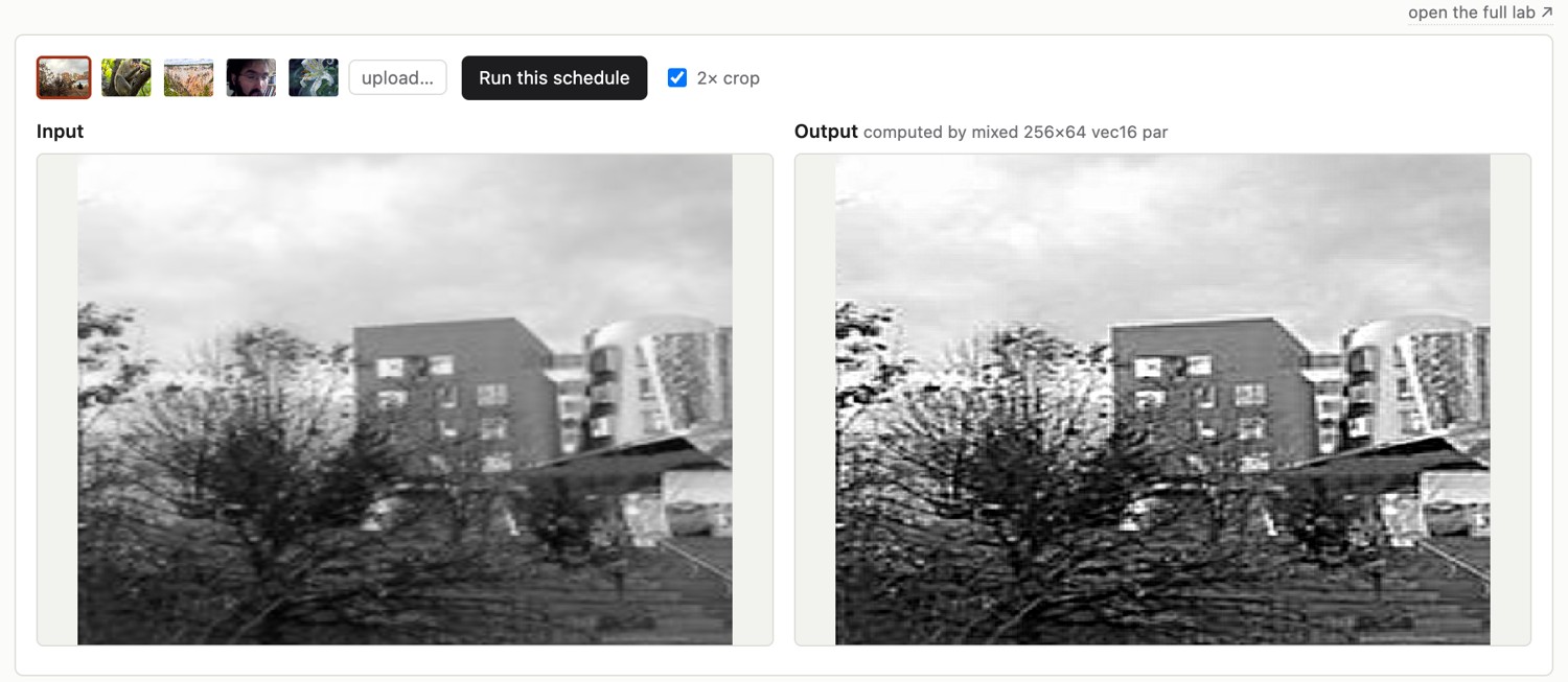
A fine tile maps to a smaller region at the next coarser level, but that region still needs a halo. As the requested interior shrinks, the halo can become a larger fraction of the work. Repeating this for many fine tiles can recompute the same coarse values repeatedly. Materializing a small coarse level once can avoid that repetition, while finer levels remain tiled. This is why the best storage decision can change with pyramid level even though every level uses a similar blur and resample operation.
29.5.7 The development loop: correctness, measurement, and benchmarking hygiene⧉
For each candidate, construct the pipeline, compile, check against a simple reference, warm up, and time repeated executions. The reference need not be inline: some updates cannot inline and deep inlining may be impractical. Compare with suitable numerical tolerances and inspect structured differences.
Run isolated candidate benchmarks sequentially when the goal is uncontended latency. Measure concurrency separately when concurrent pipelines are the intended workload. Interleave repeated baseline and candidate runs to reduce drift from clock changes and heating. For sustained camera processing, measure after the device reaches a representative thermal condition.
Searching thousands of schedules selects favorable timing noise as well as good implementations. Retest finalists in independent runs and across relevant sizes before accepting a small gain. Record compiler version, target, schedule, precision, input dimensions, and timing boundaries. An LLM can propose candidates, but the same correctness and measurement procedure applies to its suggestions.
Searching many schedules creates another measurement problem. If two schedules have the same true runtime, one can still appear faster in a noisy run. Select the minimum among hundreds of measurements and you preferentially select a favorable timing error. Re-run promising candidates independently, interleave them with a baseline, and compare their distributions before accepting the apparent gain. Stable repeats of one schedule do not establish that every extreme in a large search is real.
For isolated-kernel timing, avoid simultaneous benchmarks that compete for the same cores, cache, or memory bandwidth. For a camera application that must coexist with display or encoding work, also benchmark that intended concurrent workload. Those answer different questions. Record warmup and thermal behavior so a later, hotter run is not attributed entirely to its schedule.
29.5.8 Going farther: what the tutorials cover that we did not⧉
The official Halide tutorials cover tuples, type rules, generators, memory layouts, reduction factorization, shifted domains, and cross-compilation. Wrapper Funcs and cloned Funcs support different producer arrangements for different consumers; their semantics differ, so consult the examples before substituting one for the other.
The Halide repository's application examples include camera pipelines, local Laplacian filtering, and bilateral grids. Read their algorithms and schedules together, keeping the target and workload in view. Tracing tools can explain execution, but should be disabled during performance measurement.
The topics solve different practical problems:
- Tuples let one location return several related values, such as a weighted sum and its normalization or a maximum and its location.
- Type rules determine where arithmetic widens, rounds, saturates, or overflows. They matter before any schedule is chosen.
- Generators package a pipeline and its compilation parameters for ahead-of-time builds.
- Memory-layout constraints describe minima, extents, and strides, including planar versus interleaved color.
- Reduction predicates restrict a domain, while reduction factorization reorganizes suitable associative updates for parallel work.
- Wrapper and cloned functions allow consumers to use different producer arrangements. A wrapper introduces an intermediate use; a clone duplicates a producer definition. They are not interchangeable.
- Shifted output domains and cross-compilation separate where coordinates begin from which machine eventually runs the code.
Reading a complete application’s algorithm beside its schedule shows how these choices interact. A tracing visualization can then expose the actual execution order and storage reuse that the compact schedule requested.