12.4 Feature tracking🔗⧉

A feature track links one selected location across frames. A dense two-frame flow supplies many displacements but does not itself maintain long-term identities. Both dense and sparse trackers exist; density and temporal duration are separate design choices.

Before any of this was automatic it was done by hand, and the hand version is worth remembering because it is still in use. Rotoscoping, patented by Max Fleischer in 1915 to trace live-action footage frame by frame for animation, and reborn in visual effects as the painstaking craft of manually outlining and following an object across every frame of a shot, is tracking done by a human, one frame at a time. A rotoscope artist threads a boundary or a control point through a sequence exactly as a tracker does, but with judgment instead of a $2\times2$ matrix, which is why it is slow, expensive, and still the fallback whenever the automatic methods fail (hair, motion blur, transparency, a low-contrast edge). Everything in this section can be read as the long effort to automate the rotoscoper: detect the points worth following, follow them by brightness constancy, and flag where the tracker, like the artist, should not be trusted. Modern tools meet in the middle, with learned trackers and segmenters proposing the track and a human correcting only where they break.

12.4.1 Tracking vs dense flow: sparse-but-long vs dense-but-short🔗⧉

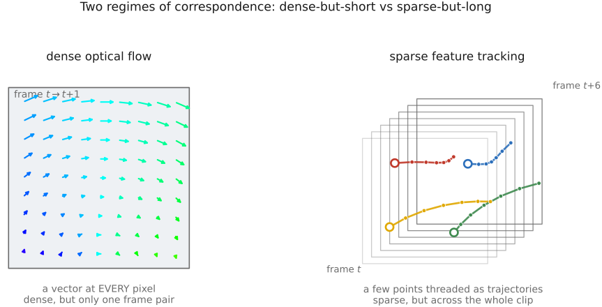
Correspondence comes in two regimes, and the distinction organizes this whole part. Dense optical flow gives a two-dimensional motion vector at every pixel, that is, a full field, but typically only between two successive frames. Feature tracking gives motion at only a sparse set of points, but threads them across a long sequence. Dense-but-short versus sparse-but-long (Figure 12.4.1⛶ fullscreen). Each is the right tool in a different regime: you reach for dense flow when you need motion everywhere (to warp a whole frame, interpolate slow motion, or segment by motion), and for tracking when you need the same physical points identified over a long clip.

Why go sparse at all? Two reasons, and they are the reasons tracking has never been retired. The first is scalability: a few hundred points carry far fewer unknowns than a million pixels. That mattered enormously when the field was young and it still matters today, for real-time SLAM and on-device tracking where you cannot afford a dense solve per frame. The second is deeper and is really about conditioning: some pixels are easier to track than others. Spend effort only where the answer is reliable, at a corner, and refuse to guess in flat regions or along edges, where the motion is ambiguous (the aperture problem you met in Chapter 12.8, Optical flow). In this light, tracking is dense flow's quality-controlled sibling: it reports motion only where it is confident, and stays silent where dense flow would be forced to hallucinate.

There is a useful label for what tracking does, made precise later in Chapter 30.1, Motion blur, temporal sampling, and resampling: tracking is the Lagrangian view of motion: "this physical point, where is it now?", following a particle through the scene. Dense per-pixel flow leans Eulerian: "at this fixed pixel, what moved through?" That Lagrangian/Eulerian dichotomy organizes the whole part, and tracking is its cleanest Lagrangian instance: it literally follows the patch rather than differentiating at a fixed location.

12.4.2 KLT = Lucas–Kanade, per feature, iterated over time🔗⧉

The workhorse of sparse tracking is the Kanade–Lucas–Tomasi (KLT) tracker, and its definition is simple: take the Lucas–Kanade patch solve from Chapter 12.8, Optical flow, apply it to one small window around a feature, iterate it to convergence, then repeat for the next frame. That is the entire algorithm. The lineage factors the credit cleanly: Lucas & Kanade (1981) gave the iterative registration update; Tomasi & Kanade 1991 packaged that update as a feature tracker; and Shi & Tomasi (1994) settled which features to track. KLT is the assembly of those three.

The per-patch system is pure reuse: it is Lucas–Kanade restricted to a window $W$, so we will set it up but not re-derive it. Assume every pixel in the window shares one displacement $\mathbf{u}=(u,v)$, and stack the brightness-constancy constraint $I_x u + I_y v + I_t = 0$ over all the pixels in $W$. That is an over-determined linear system in two unknowns, and its least-squares normal equations are

so the displacement update is formally

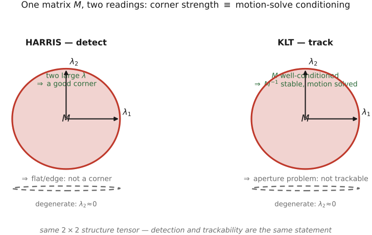
Now look hard at that $2\times2$ matrix $M$. It is exactly the structure tensor of Harris Harris & Stephens 1988 (the second-moment matrix of gradient products, Gaussian-weighted over the window), the very object that classifies a patch as flat, edge, or corner in Chapter 12.3, Sparse matching. The same matrix, no new math. The whole detection apparatus from corner finding turns out to be precisely the apparatus the motion solve needs (Figure 12.4.2⛶ fullscreen). Lucas–Kanade imposes a shared displacement over a window; Horn–Schunck Horn & Schunck 1981 instead couples a field through a smoothness penalty. They use the same brightness linearization but solve different models.

One iteration is not enough, and the reason is built into the derivation: brightness constancy was Taylor-linearized, so a single solve is only valid for sub-pixel motion. The fix is Gauss–Newton on the patch sum-of-squared-differences: warp the second-frame patch by the current estimate $\mathbf{u}$, recompute the temporal difference $I_t$ on the warped patch, re-solve for a residual $\Delta\mathbf{u}$, add it, and repeat until the residual is negligible (the inverse-compositional account of Baker & Matthews 2004 unifies the bookkeeping).

That handles small motion; real videos move farther than a pixel between frames. The standard remedy is the same coarse-to-fine logic as dense flow, now localized to each feature: run the iteration down a pyramid (Bouguet, 2000). Solve on a heavily blurred and downsampled level, where the displacement is small enough for the linearization to hold; propagate that estimate as the initial warp for the next-finer level; refine; repeat to full resolution.

Finally, thread it through time. Having localized the feature in frame $t{+}1$, use that location as the starting guess for frame $t{+}2$, and so on down the clip. KLT is this tiny $2\times2$ solve threaded greedily through the whole video, one small matrix inverse per feature per frame, almost free. Assembled, the three layers (iterate to converge, thread to the next frame) read as one short loop:

for each active feature with current position p:
    d = predicted displacement from this frame to the next
    repeat up to max_iterations:
        compare current-frame patch at p with next-frame patch at p+d
        use valid samples to build the consistent Jacobian and residual
        if information matrix is poorly constrained: mark lost; stop
        solve the small least-squares system for delta
        d = d + delta
        if delta is small and residual is acceptable: stop
    if fit passes visibility and consistency checks:
        p = p + d
        report position p and keep d as a motion prediction
    else:
        mark track lost; retain its history without inventing a position

But "greedy and memoryless" is exactly the property that makes drift and occlusion bite, as we will see two sections on.

12.4.3 Good features to track = where the structure tensor is well-conditioned🔗⧉

Here is the hinge the whole section turns on. The update $\Delta\mathbf{u}=M^{-1}\mathbf{b}$ is only meaningful when $M$ is invertible and well-conditioned, meaning you can actually trust the inverse. And the conditioning of $M$ is read straight off its eigenvalues $\lambda_1\ge\lambda_2$, the same eigenvalues that, in the Harris derivation, sort a patch into flat, edge, or corner. So the question "is this a good feature to track?" is literally "is the tracking matrix well-conditioned?", which is in turn literally "is this a corner?" One question in three forms.

Walk through the three cases. They are exactly the Harris partition, now read as trackability:

• Flat region ($\lambda_1\approx\lambda_2\approx 0$). The window has no texture, so $M$ is near-zero and $M^{-1}$ blows up. The motion is totally ambiguous because every direction looks the same. Untrackable.
• Edge ($\lambda_1\gg\lambda_2\approx 0$). $M$ is rank-deficient: motion along the edge is unconstrained, and you can recover only the across-edge component. This is the aperture problem in its purest form. Only half the motion is recoverable, and the unrecoverable component is what drifts.
• Corner ($\lambda_1,\lambda_2$ both large). $M$ is well-conditioned and the motion is fully determined in both directions. Trackable.

The selection rule falls right out of this. Shi & Tomasi's (1994) "good features to track" criterion is the simple, principled test

read as: require the smaller eigenvalue to be large enough, that is, demand that both directions be well-constrained, not just one. This is nothing but the conditioning of $M$ stated directly, and it is the same $\min(\lambda_1,\lambda_2)$ corner response cross-referenced in Chapter 12.3, Sparse matching. The Harris response $R=\det M - k\,(\operatorname{tr} M)^2$ is a determinant-and-trace proxy for the same quantity. What matters is the direction of the logic: the detector and the tracker agree by construction, because Shi & Tomasi derived "what makes a good feature to detect" from "what makes a good feature to track", not the other way round (Figure 12.4.3⛶ fullscreen).

In practice the recipe is exactly the Harris pipeline: compute $M$ over a window at every pixel (image gradients → pointwise products → Gaussian-weighted sum), score each pixel by $\min(\lambda_1,\lambda_2)$, non-maximum-suppress, and keep the top-$N$ well-spread points. Those are the features you then KLT-track.

One real tension governs the window size, and it is the recurring small-versus-large-aperture trade of every patch method. A small window localises precisely but sees little texture, so $M$ is poorly conditioned and noise fools it. A large window is better conditioned but spans multiple motions: across a depth discontinuity or an object boundary, a single displacement $\mathbf{u}$ no longer fits the whole window. The sweet spot trades localization against conditioning.

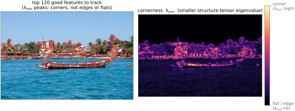
The minimum eigenvalue measures the weakest direction's absolute information, while the eigenvalue ratio measures conditioning. They are related but different: a matrix proportional to the identity can be perfectly conditioned and still carry almost no information if both eigenvalues are tiny. With a fixed noise and derivative convention, a minimum-eigenvalue threshold rejects that case. Large values also do not rule out a wrong correspondence on repeated texture.

12.4.4 What breaks long-term tracking: drift, appearance change, occlusion, and re-detection🔗⧉

A single small patch tracked greedily over a long video is not enough, and the failures are predictable. There are three of them, and one standard response.

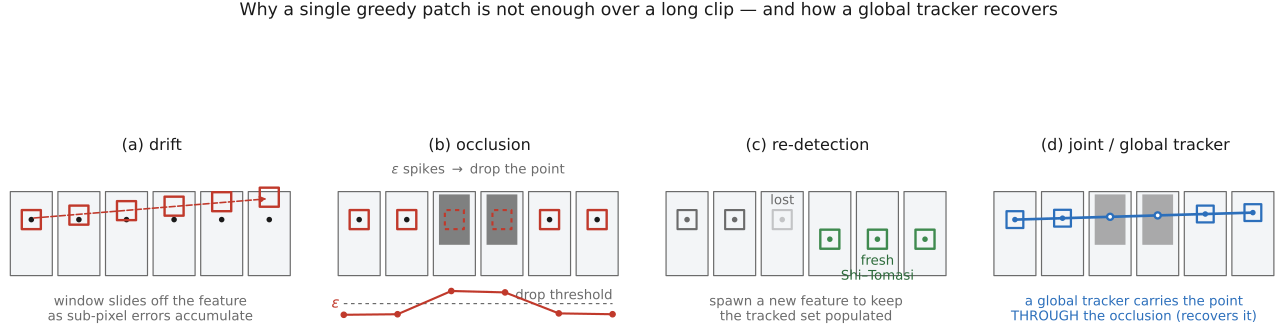
Drift: the cost of greediness. Each frame's tiny Lucas–Kanade (LK) residual is imperfect, and chained over hundreds of frames the sub-pixel errors accumulate until the window has slowly slid off the true feature, so sub-pixel bias becomes whole pixels (Figure 4a). The classic remedy is to anchor to the first frame: match against the original template from frame $t_0$ rather than the previous frame, so the error does not compound. But anchoring trades one problem for another, because over a long clip the template goes stale.

Appearance change: the template goes stale. Over many frames the patch changes: lighting shifts, the object undergoes out-of-plane rotation, its scale changes as it nears or recedes, perspective skews it. A pure-translation match against a fixed template degrades. Shi & Tomasi's answer is a two-speed scheme: track plain translation frame-to-frame (small motion, cheap) but verify against the anchor template with an affine warp, allowing the patch to rotate, scale, and shear when you check whether it is still itself. The affine dissimilarity

measures how well the current patch still matches its origin under the best affine warp $A$ (with translation $\mathbf{d}$). A large $\varepsilon$ means the feature is no longer the thing you started tracking.

Occlusion or leaving the frame removes a visible correspondence. A shadow or specular change can instead break the appearance model while the surface point remains visible. In both cases a tracker may drift to an unrelated patch; use validity, residual and consistency checks rather than reporting every update as a valid track.

Re-detection: keep the set populated. As features bleed away to drift, occlusion, and leaving the frame, periodically re-run Shi–Tomasi and spawn fresh features in the gaps, so the tracked set stays dense enough and well-distributed (Figure 4c). Detection and tracking become an interleaved loop rather than a one-shot detect-then-track pipeline.

Step back and the plain limitation is clear, and it is what motivates the next section. Classical KLT is per-point, greedy, and forgetful: each feature is tracked independently, with no memory of where it went and no way to recover a point once it reappears from behind an occluder. Points also drift relative to one another, with no enforced global consistency. These are exactly the failures the learned trackers were built to fix.

12.4.5 Modern point trackers (briefly)🔗⧉

The failures of greedy KLT have a modern answer, and it is a clean instance of L7.6show: the bitter-lesson successor keeps the task, "track this physical point through a video, even through occlusion," but replaces the hand-built brightness patch with learned features and the greedy per-frame solve with a learned iterative update, trained on synthetic video with ground-truth tracks. The classical scaffolding survives as architecture: a cost volume of appearance similarity, iterative refinement of the trajectory, and now an explicit visibility / occlusion prediction. The skeleton Lucas, Kanade, and Tomasi laid down is intact; only the operator is fit to data. We sketch the family here and leave the full models to Chapter 7.3, Deep learning.

• PIPs (Particle Video Revisited) (Harley et al., 2022) tracks one point at a time over a temporal window, solving jointly for its $(x,y)$ location and an appearance vector across all frames, predicting visibility per frame, and initializing with a constant location and appearance that it then iteratively refines (RAFT-style; see RAFT in Chapter 12.8, Optical flow). It reintroduces the long-range, occlusion-aware particle tracking that KLT lacked.
• TAP-Vid (Doersch et al., 2022) Doersch et al. 2022 (TAP-Vid) frames the modern task (Track Any Point) and, just as important, supplies the benchmark that made progress measurable. As with optical flow, the long-standing bottleneck was ground-truth data.
• CoTracker (Karaev et al., 2023) Karaev et al. 2023 (CoTracker) makes the key move: tracking points jointly beats tracking them independently. Points on the same object constrain one another, which buys global consistency and much better occlusion handling, where a point hidden behind an object can be inferred from its visible neighbors. Mechanically it is a transformer over a sliding window with attention factorized across space, time, and the group of tracks, iteratively updating each track's position, appearance, and visibility (with extra "register" tokens giving the network scratch space so it does not hijack real pixels).

Modern point trackers use temporal context, learned appearance and visibility estimates to reduce drift and reconnect tracks. Occlusion and out-of-domain motion remain difficult. Evaluate identity errors and recovery after occlusion, not just average position error on visible easy frames.

12.4.6 An application: synthetic motion blur from a track🔗⧉

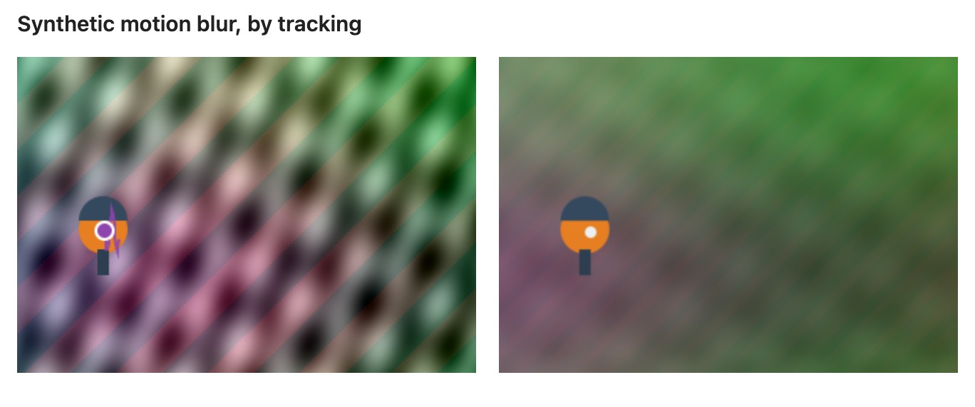
One application shows the mechanics directly (Figure 12.4.5⛶ fullscreen). A long exposure that pans with a moving subject, leaving the subject sharp and the background streaked, is hard to capture in camera. But you can manufacture it from an ordinary short clip: track a point on the subject, stabilize every frame so that point holds still (translate each by the negative of the tracked displacement), and average the stabilized frames. Content whose image motion is well described by that same translation remains sharp; rotation, deformation or depth-dependent motion can still blur the subject; everything moving relative to it integrates into a streak, which gives the panning blur, anchored wherever you chose to track. It is the temporal mirror of denoising-by-averaging from Chapter 13.2, Denoising by averaging: there you align frames to remove the differences (noise); here you align to one point so the remaining motion is kept, as blur.