31.1 Light fields 101⧉
The world does not look the same from every vantage; a scene radiates a different image in every direction, and our two eyes, separated by a few centimeters, already exploit the difference to see depth. A single photograph collapses all of that into one frozen view. The question of this part is what we would have to record to keep it all, and the answer is a clean, finite object: the light field.
We have actually been circling it for several chapters. In Chapter 2.3, Lens Image formation a lens gathers a whole cone of rays leaving one scene point and bends them back to a single point on the sensor; in Chapter 2.4, Image measurements as integrals over the plenoptic function we said plainly that a pixel value is an integral: it sums the light arriving over the pixel's area and over the aperture's solid angle, and reports one number. This chapter takes that integral seriously and asks what is inside it. The light hitting the sensor is not one number per pixel; it is a bundle of rays, each carrying its own radiance, each having traveled a different path through the aperture. The pixel throws their distinctions away. The light field keeps them.
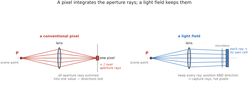
A conventional pixel is the integral over all the rays that cross the aperture and converge there; which rays converge where is exactly what focus sets. Record the rays themselves instead of their sum, and you defer the irreversible capture decisions, such as focus, aperture, and even viewpoint, until after exposure. You pay with far more data and a harder reconstruction, and in return any conventional photograph becomes a projection you compute after the shutter. This is the same capture-the-full-set-decide-later move as HDR (the exposure axis) and focus stacking (the focus axis, Chapter 23.3, Focal stacks and depth of field extension); here the axis is the aperture/angle, the full set of rays.
31.1.1 Capture rays, not pixels⧉
Start with the single point that a lens brings to focus. Every ray that leaves that scene point and falls anywhere on the lens aperture is bent so that it lands on the same sensor location. That convergence is what "in focus" means, and we drew it in Chapter 2.3, Lens Image formation. The sensor pixel sitting there does not see the rays one at a time. It accumulates them. Its value is
an integral over the cone of aperture rays that converge at the pixel. In words: a pixel is the sum of all the rays crossing the aperture that the lens steered onto that spot. When the point is in focus the cone is tight and the rays agree; when it is out of focus they land smeared across a disc, the circle of confusion, and neighboring pixels integrate overlapping cones. Either way the pixel reports one number and the individual rays are gone.
Now the move. Do not perform the integral. Keep each ray as its own measured quantity, its radiance tagged with the direction it came from, and what you hold is no longer an image but a function over rays. From that function you can re-do the integral any way you like: sum the cone that focuses at this depth and you get one photograph; sum the cone that focuses at that depth and you get another; sum only the rays through the center of the aperture and you get a sub-aperture image with greater geometrical depth of field, still limited by sampling, diffraction, and finite angular acceptance. The single captured object contains a continuum of conventional photographs, and you choose among them afterward. That is the promise, and the rest of the chapter is about how to index the rays so the bookkeeping is clean (Figure 31.1.1).
31.1.2 The plenoptic function, reduced to four dimensions⧉
How many numbers does it take to name "all the light, everywhere, going every way"? Adelson and Bergen answered this with the plenoptic function Adelson & Bergen 1991: stand at any point in space, look in any direction, and there is a radiance. Tally the degrees of freedom and you get seven: three for the eye's position $(x,y,z)$, two for the viewing direction $(\theta,\phi)$, one for wavelength $\lambda$, one for time $t$. The plenoptic function $P(x,y,z,\theta,\phi,\lambda,t)$ is the complete record of everything any eye or camera could ever see, from anywhere, looking anywhere, in any color, at any instant. It is the most general thing there is to capture, and at seven dimensions it is also hopeless to store.
It collapses fast, and the collapse is physical, not a convenience. Freeze a color channel and an instant and drop $\lambda$ and $t$; that leaves five. The decisive reduction is the next one: along a ray in free space, radiance is constant. Light traveling through empty air between the scene and the camera does not change as it goes. Once you know a ray's radiance at one point along it, you know it everywhere along it, and the third position coordinate becomes redundant. Where you sample the ray no longer matters; only which ray you mean. A ray in 3-D is fixed by four numbers, and the plenoptic function for a camera in free space collapses to the 4-D light field.
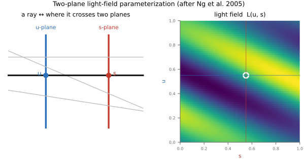
The cleanest way to name a ray with four numbers is the two-plane parameterization of Levoy and Hanrahan Levoy & Hanrahan 1996 and, concurrently, the Lumigraph of Gortler and colleagues Gortler et al. 1996: put down two parallel planes and record, for each ray, where it pierces each one. Take one plane at the lens aperture, with coordinates $(u,v)$, and one at the focal/sensor plane, with coordinates $(s,t)$. A ray punches through the first plane at $(u,v)$ and the second at $(s,t)$, and those four numbers pin it down completely. The light field is the function
the radiance of the ray that passes through aperture point $(u,v)$ and image point $(s,t)$. In words: every ray is a point in a 4-D space, two coordinates for where it crosses the aperture and two for where it crosses the image plane. A conventional photograph is then a 2-D slice or a projection of this 4-D object, which is the unifying picture for everything that follows (Figure 23.3.7).
A pair of caveats, because the literature is not uniform. First, a coordinate-convention problem: different authors place the two planes differently and label the coordinates differently, for example $(u,v,s,t)$ or $(s,t,u,v)$, with aperture-first or image-first order, planes at the lens or planes straddling the scene, so a formula copied from one paper rarely drops cleanly into another. The idea is invariant; the coordinates are a convention you must pin down before you compute. Second, the parameterization is not perfectly uniform: equal steps in $(u,v,s,t)$ are not equal steps in ray direction except in the paraxial approximation (rays close to the axis, small angles), and away from the axis the sampling stretches. For building intuition the two planes are exactly right; for a calibrated reconstruction you carry the non-uniformity as a correction.
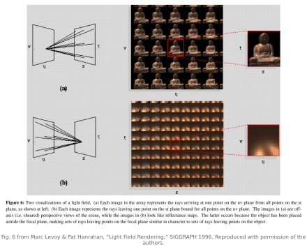
The two-plane diagram is a schematic; the object it names is real, and the original paper drew it as an array of actual captured sub-images (Figure 31.1.2). Reading that array against the diagram makes the abstraction tangible: hold the aperture point fixed and the array becomes a grid of pinhole views; hold the image point fixed and it becomes a grid of angular views of the same object.
31.1.3 Ray and point are dual⧉
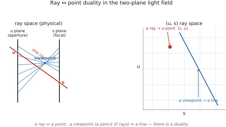
Live in the 2-D simplification for a moment, where each plane contributes one coordinate and ray space is the flat picture $(u,s)$. Drop $v$ and $t$, draw the aperture line and the image line, and watch what familiar objects become.
A single ray crosses the two lines at one $u$ and one $s$, so it is one point $(u,s)$ in ray space. That is the picture from the last figure. Now consider a viewpoint: a single point in the world (or a single pinhole the camera could look through) emits, or admits, a whole pencil of rays fanning out in every direction. Each of those rays has its own $(u,s)$. As you sweep through the pencil, the aperture crossing $u$ and the image crossing $s$ change together and in lockstep. By similar triangles, a viewpoint at a fixed depth ties $s$ to $u$ by a straight linear relation. So the pencil of rays through one point traces out a straight line in ray space.
That is a genuine duality, and it comes straight from the Lumigraph reading of light fields Gortler et al. 1996: in ray space, a ray is a point and a viewpoint is a line. The two pictures swap. It is the same kind of point–line duality that runs through projective geometry, and it is more than a curiosity: the slope of the viewpoint's line in ray space encodes how far away that point is, which is the seed of every depth and refocusing trick in this part. Lines in ray space encode depth (Figure 31.1.3).
31.1.4 Reading the 4-D structure through its 2-D slices⧉
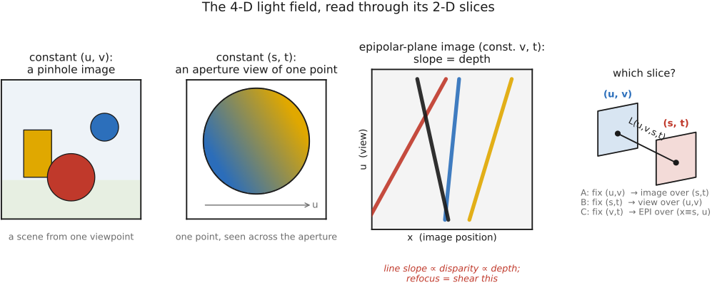
Four dimensions is one too many to draw, so we understand the light field the way we understand any high-dimensional object: we slice it, fix some coordinates and look at the 2-D image of the rest. Three slices carry the whole intuition, and each one is a familiar object in disguise.
Fix the aperture point $(u,v)$ and sweep $(s,t)$. You are holding the ray's entry on the lens plane still and letting its image-plane crossing range over the whole sensor. That is exactly the set of rays through one point of the aperture, which is a pinhole image. Every $(u,v)$ gives you a slightly different pinhole view of the scene, taken as if the camera were a pinhole at that spot on the lens. Step $(u,v)$ across the aperture and these views shift in parallax: near things slide against far things, the apple's highlight migrates. This is the slice that holds the "look around the scene" content.
Fix the image point $(s,t)$ and sweep $(u,v)$. This fixes an image-plane coordinate, not generally one scene point. For a point on the plane to which the views have been aligned, aperture samples observe that point from different angles; away from that plane they can observe different surface locations. This 2-D slice is an aperture view or angular view of that single point: how its color and brightness change with viewing direction. For one unoccluded Lambertian point, correctly aligned across views under fixed illumination, radiance is independent of viewing direction. Depth mismatch and occlusion can make the fixed-coordinate slice vary even for matte surfaces. For a glossy or specular surface it is not. The highlight lives at particular angles, and the aperture slice captures it. And the shape of this variation depends on depth, because where a scene point's rays land on the sensor as you move across the aperture is governed by how far away it is.
Fix one image row and one aperture row: the epipolar-plane image. This is the slice that ties it all together. Hold the vertical image coordinate $t$ at one value (pick a single row $y$ of the picture) and the vertical aperture coordinate $v$ at one value (a single horizontal strip of viewpoints), and let $s$ and $u$ vary. The resulting 2-D image, with horizontal image position against horizontal aperture position, is the epipolar-plane image, or EPI. By the duality of the previous section, a scene point becomes a straight line in the EPI, and its slope encodes that point's depth: slope varies with depth according to the chosen coordinate system. Opposite signs occur on opposite sides of a chosen zero-disparity plane, not simply because points are “near” and “far.” Read an EPI and you are reading disparity directly off the picture. And here is the connection that runs to the next chapters: refocusing is a shear of the EPI. Slant the whole slice so that the lines of one chosen depth become vertical (zero disparity), integrate across $u$, and that depth snaps into focus while the rest blurs. The EPI is where ray space, depth, and refocusing are visibly the same object (Figure 31.1.4).
31.1.5 Rendering a new view by looking up rays⧉
The reason the two-plane representation is worth its storage is that rendering out of it is direct. Suppose you want a photograph from a viewpoint the camera never physically occupied, namely a new pinhole camera placed somewhere in front of the scene. You do not re-render the world; you re-index the rays you already have.
For each pixel of the desired new view, trace the ray from the new camera's center through that pixel out into the scene. That ray crosses the aperture plane at some $(u,v)$ and the image plane at some $(s,t)$, four numbers in all, and the color of the pixel is just the stored radiance $L(u,v,s,t)$. Read it back: to make a new image, shoot a ray per output pixel, intersect it with the two planes, and look up the light field there. For a continuous field covering the requested rays, no scene geometry is needed; the rays are the scene, and synthesizing a view is a lookup. This is the original "light-field rendering" of Levoy & Hanrahan 1996 and the Lumigraph's view reconstruction Gortler et al. 1996.
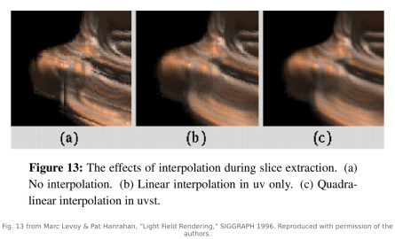
The catch is resampling. The ray you trace will almost never pierce the two planes at exactly the $(u,v,s,t)$ where you have a stored sample; it lands between samples, so you must interpolate among the nearby recorded rays. Coarse angular sampling (too few $(u,v)$) shows up as ghosting, a faint double image, because the in-between rays you needed were never captured and the interpolation guesses badly. Whole sub-fields are devoted to interpolating ray space well, and the Lumigraph's contribution was precisely to use a little approximate scene geometry to steer the interpolation. For now, with the rays in hand, a new viewpoint is a per-pixel ray lookup, and the only hard part is filling the gaps between the rays you actually measured (Figure 31.1.5).
31.1.6 Light fields vs. plenoptic and radiance⧉
One closing caution about the object we have built, because it matters for the analyses to come. The two-plane light field $L(u,v,s,t)$ is a parameterization, a convenient set of coordinates for naming rays, not the physical quantity itself. The physical quantity is radiance along rays, the plenoptic function reduced to free space; it lives on the space of rays, which has its own natural geometry, independent of any planes we choose to lay down. And the two-plane coordinates are not uniform on that space: equal steps in $(u,v,s,t)$ do not correspond to equal steps of ray position-and-direction except in the paraxial limit (small angles near the axis). A near-axial ray and a steeply tilted one occupy the same-sized cell in $(u,v,s,t)$ yet very different-sized regions of the true ray space. Each light-field sample therefore carries a different density, a different measure.
The distinction matters when converting coordinate integrals into physical irradiance: the measure includes geometric weights and the chosen parameterization’s Jacobian. It does not make a Fourier transform in two-plane coordinates invalid away from the optical axis. Such a transform is mathematically well defined for that coordinate signal, and a shear or projection theorem can be exact for its stated model. Paraxial approximations enter particular lens and radiometric models, not the existence of the Fourier transform. State the coordinates, physical weights, and optical assumptions separately.
That closes the foundational picture. We have an object, the 4-D light field $L(u,v,s,t)$, and we know how to read it (slices), what its geometry means (ray↔point duality, depth as slope), and how to make any conventional photograph out of it (trace, intersect, look up). Two questions remain, and they are the next two chapters. How do you physically capture all those rays in one shot? That is the light-field camera. And once you have them, how do you refocus and change aperture after the fact? That is shift-and-add. Both simply re-do the integral from this chapter after the shutter.
Recap: big lessons of this chapter
A conventional pixel is the integral over all the rays that cross the aperture and converge there; which rays converge where is exactly what focus sets. Record the rays themselves instead of their sum, and you defer the irreversible capture decisions, such as focus, aperture, and even viewpoint, until after exposure. You pay with far more data and a harder reconstruction, and in return any conventional photograph becomes a projection you compute after the shutter. This is the same capture-the-full-set-decide-later move as HDR (the exposure axis) and focus stacking (the focus axis, Chapter 23.3, Focal stacks and depth of field extension); here the axis is the aperture/angle, the full set of rays.