22.2 Aberrations correction⧉
Every aberration in Chapter 22.1, Aberrations and optical challenges, including spherical aberration, coma, astigmatism, field curvature, distortion, and axial and lateral chromatic aberration, can be reduced, and the cures fall into two complementary families. You can fight the defect in the glass, by shaping and combining elements, choosing glasses, and stopping down; or you can let the optics get only close and finish the job in software, by remapping, rescaling, and deconvolving in the image-signal processor. This chapter takes the two families in turn. It develops the part's main tradeoffs, partly in optics and partly in computation.
22.2.1 The two families of cure⧉
The descriptions are settled; what is left is the engineering. A useful way to organize it is by what the defect did to the light, because that decides which family of cure can reach it. Distortion and lateral chromatic aberration primarily misregister image positions, while vignetting attenuates the signal. Warping and gain correction can compensate these effects, at the cost of resampling and amplified corner noise, and increasingly the optics is designed expecting that. Blur defects, including spherical aberration, coma, astigmatism, and axial chromatic aberration, genuinely spread a point into a blob, which is much harder to undo after the fact; they are fought first in glass (the right surface shapes, the right glass pairings, a smaller aperture) and only what the glass leaves behind is handed to a calibrated deconvolution. So the chapter goes glass first, then computation, and within each, the cures are organized by the defect they target, because in a real lens, each element, surface, and glass choice usually influences several aberrations at once.
22.2.2 Correction in glass⧉
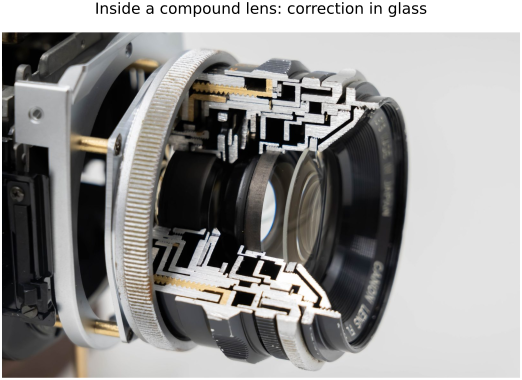
The first line of defense is the optics itself, and the strategy is always the same: add free parameters until you have enough to cancel the aberration you care about. In practice that means a well-corrected photographic lens is usually a compound system: a column of several curved elements in groups, and cutting one open shows the machinery directly (Figure 22.2.1). Four classic moves cover almost all of it.
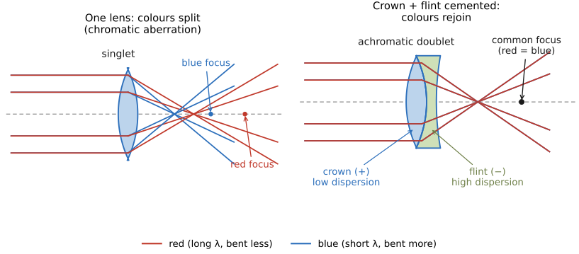
The headline move for color is the achromat, the cemented crown-plus-flint doublet that is the minimum system able to correct chromatic aberration. The idea is to make the dispersion of two elements cancel while their focusing power adds. Pair a positive (converging) element of low-dispersion crown glass with a negative (diverging) element of high-dispersion flint glass. The crown does most of the focusing; the flint, being weaker in power but stronger in dispersion, undoes the crown's color spreading without undoing all of its focusing. Quantitatively, if the two thin elements have powers $\phi_1, \phi_2$ (power $=1/f$) and Abbe numbers $V_1, V_2$ (the dispersion measure $V_d=(n_d-1)/(n_F-n_C)$ defined in Chapter 22.1, Aberrations and optical challenges), the primary longitudinal color between the selected wavelengths cancels, in the thin-element contact approximation, when
the achromat condition: the powers, each weighted by the glass's dispersion (divided by its Abbe number), sum to zero. Since $V_1, V_2 > 0$, the two powers must have opposite sign: one converging and one diverging, which gives the familiar positive-crown/negative-flint positive achromat when $V_1>V_2$. Negative achromats, air-spaced pairs, and other glass combinations also exist. Solving the condition jointly with the requirement that the total power $\phi_1 + \phi_2$ hit the desired focal length pins down both elements. An achromat makes two wavelengths (say blue $F$ and red $C$) share a focus exactly, with the in-between green error (the residual secondary spectrum) reduced to a tiny fraction of the original. As a bonus, the extra surfaces let the designer also tame the doublet's spherical aberration, which is why the achromatic doublet is the workhorse front element of so many lenses.
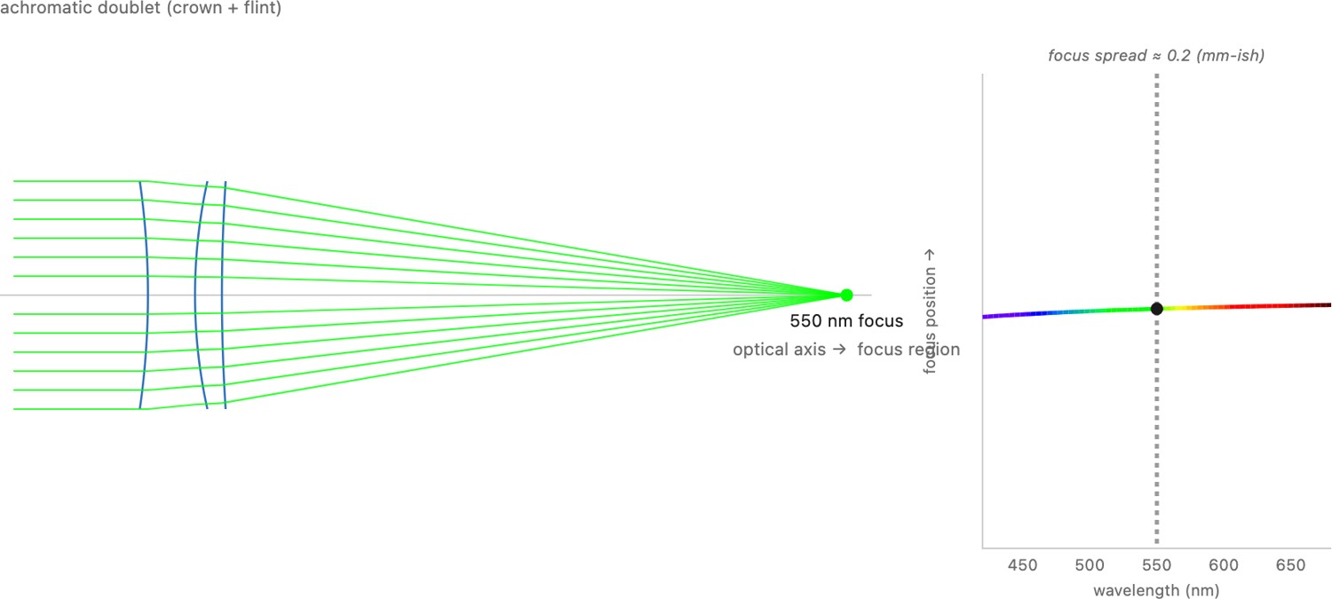
When two wavelengths are not enough, as in long telephotos and astrophotography where the residual secondary spectrum is visible as a faint color halo on highlights, the apochromat (or superachromat) corrects three or more wavelengths at once. This needs glasses with unusually favorable dispersion curves: extra-low-dispersion (ED) glass, special-dispersion "fluorite-equivalent" glasses, or actual fluorite (calcium fluoride) crystal, which has both very low dispersion and an anomalous dispersion curve that lets the designer flatten the color error across the whole visible band. ED elements are why a modern super-telephoto can render a backlit bird's feather edges without a magenta-and-green seam; they can be expensive; white barrels on some telephotos address solar heating rather than identifying the glass type, which is precisely the kind of cost that motivates handing the residual to software instead.
A wholly different way to bend color the right direction is diffraction rather than refraction. A diffractive (kinoform) surface, a fine concentric microstructure etched into one face, focuses by interference, and its power is linear in wavelength, the opposite sign of glass and far stronger: its effective Abbe number is about $-3.45$, against $+30$ to $+85$ for glass. So a tiny diffractive correction etched onto an ordinary singlet cancels that singlet's color with one element instead of a cemented pair. This is the principle behind Canon's DO (diffractive optics) and Nikon's PF (phase Fresnel) telephotos, which are dramatically shorter and lighter than the equivalent all-glass apochromat. The interactive figure below traces real rays through all three cures so you can watch the focus spread collapse.
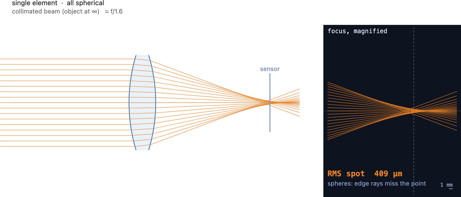
The headline move for spherical aberration is the aspheric element. As described in Chapter 22.1, Aberrations and optical challenges, a spherical surface focuses its edge rays short; an aspheric surface, whose profile departs from a sphere by a designed polynomial, gives the designer an extra knob to kill spherical aberration (and to flatten the field) with far fewer elements than the alternative of splitting power across many spherical surfaces. This is the enabling technology of compact fast primes and especially of cell-phone cameras, whose tiny stacks of five-to-eight molded elements would be impossible with spheres alone. There is a manufacturing sidebar worth keeping: spherical surfaces are easy to make precisely because any two surfaces ground together with abrasive between them naturally wear toward a sphere: geometry hands you the sphere for free. Aspheres lack this convenient spherical generating process. They can be ground and polished, diamond-turned where the material permits, or precision-molded by pressing glass or plastic against a figured die. That is exactly why cheap molded plastic and glass aspheres were the breakthrough that gave phone cameras their optical edge: the surface that is hardest to grind is easy to mold in volume.
Finally, the fix that costs nothing and adds no glass: stopping down. Most of the aberrations that matter, including spherical aberration, coma, and the optical part of vignetting, scale with how far out in the aperture the offending rays travel, so closing the iris to use only the well-behaved central zone reduces their contribution together. Primary lateral color and distortion do not generally disappear on stopping down. This is why nearly every lens is sharpest a couple of stops down from wide open rather than at its maximum aperture. The catch, from FUNDAMENTALS, is that you cannot keep stopping down forever: at small apertures diffraction takes over and softens everything, so there is a sweet spot, often below full aperture but dependent on the lens, field point, and metric, where the aberrations have shrunk but diffraction has not yet bitten. Beyond it, closing further trades aberration blur for diffraction blur and the image gets worse. Stopping down is the photographer's blunt instrument; the precise fixes live in the glass, and what neither the glass nor the iris can reach economically is handed to computation.
22.2.3 Computational correction⧉
Everything above fights the aberration in the optics. The computational-photography move is to let the optics get the image only close and finish the job in the image-signal processor (ISP), shifting the design's operating point on the cost-versus-quality front (cross-ref Chapter 22.4, Lens optimization). Two tools do the bulk of it, and they map cleanly onto the two kinds of aberration: geometric (a sharp image in the wrong place) versus blur (light spread out of place).
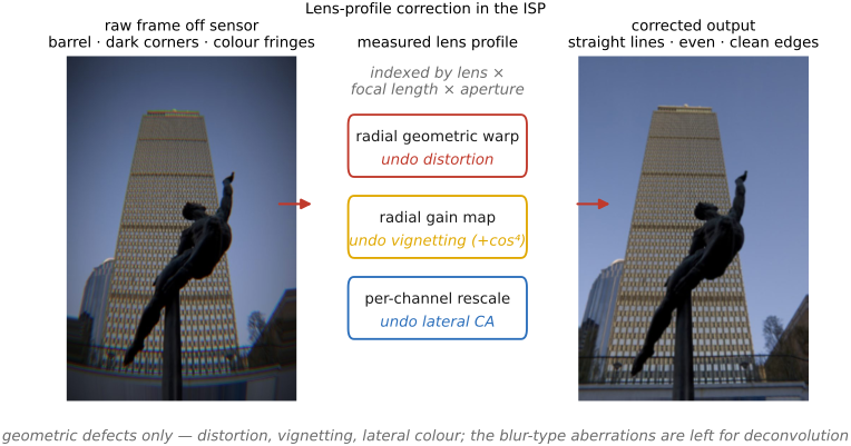
The first tool is lens-profile correction, and it handles all three of these profile-correctable effects. For each lens, and for each combination of focal length, aperture, and focus distance, the manufacturer or a community database measures a profile: a table of how that lens distorts, vignettes, and color-fringes. Then the ISP simply plays the profile in reverse on every frame. Geometric distortion is undone by a radial warp, resampling each pixel along a corrective function of its distance from center, $r' = r\,(1 + k_1 r^2 + k_2 r^4 + \cdots)$. The direction of this map must be specified: a forward Brown–Conrady polynomial maps undistorted coordinates to distorted source coordinates, which is exactly what output-to-input resampling needs. Its mathematical inverse is not generally another polynomial with negated coefficients. Resampling restores geometry but can change sharpness, crop the image, and stretch corner samples. Vignetting is undone by a radial gain map, brightening the corners back to the center's level. The same map corrects both the lens's optical vignetting and the FUNDAMENTALS $\cos^4$ falloff in one pass (cross-ref the natural-illumination falloff there). Lateral CA is undone by rescaling each color channel radially about the center by the tiny per-channel factor the profile records, collapsing the red-to-blue fringe back to a single edge. All three are widely used, particularly in camera-generated images, though raw converters and lens combinations differ in which profiles they apply. Phone lenses in particular are designed expecting this correction, deliberately leaving in heavy barrel distortion (it lets the optics be smaller and faster) on the understanding that software will straighten it. This is routine optics-plus-computation.
The second tool reaches the blur-type defects, and it is where this chapter rejoins the deblurring machinery from the single-image part. An aberrated lens does not just displace points. For spherical aberration, coma, astigmatism, and axial CA, it genuinely spreads each point into a small blob, the lens's point-spread function (PSF). The forward model is the one convolution we keep returning to: within a small region with approximately constant PSF, the recorded image is the ideal scene convolved with that PSF, plus noise,
Here $x$ is the ideal image, $k$ the local PSF, $n$ the noise, and $y$ the observation. Across the full frame, use a space-varying operator $y(p)=\sum_q k(p,q)x(q)+n(p)$ rather than one convolution.
If we know the PSF, we can try to invert that convolution, by deconvolution, and recover the sharp scene. And for a known lens we can know the PSF, by measuring it (shoot a point source or a calibration target through the lens). This difference from blind motion deblurring matters: here the kernel is calibrated, not guessed, so the inversion is a non-blind deconvolution, the easier problem. It uses exactly the regularized-inverse toolbox from Chapter 6.3, Linearity, Fourier, aliasing and deblurring, the Wiener filter prototype
where $X,Y,K$ are Fourier transforms and $\mathrm{SNR}^{-1}=S_n/S_x$ is the ratio of noise and signal power spectra at that frequency. This is not the local amplitude SNR used in the noise chapter. The filter at each frequency divides the blur back out where there is signal worth recovering and suppresses frequencies where the lens left too little signal relative to noise. The one twist particular to lenses is that the PSF is spatially varying (it is tight in the center and grows comatic and stretched toward the corners), so the deconvolution must use a different kernel per region of the frame, a calibrated map of PSFs rather than one global blur. Kee et al. Kee, Paris et al. 2011 (spatially-varying optical blur) do exactly this end to end: calibrate a lens's spatially-varying PSF across the field (and across zoom/aperture) and remove the resulting optical blur by per-region non-blind deconvolution.
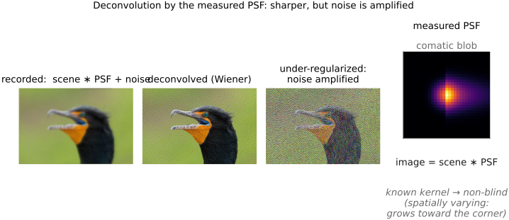
The limits are the same as in any deblurring problem. Deconvolution amplifies noise at exactly the frequencies the lens attenuated most, its modulation transfer function (MTF) dips toward zero there, so it can sharpen what was merely attenuated but cannot recover what was destroyed: information the optics drove below the noise floor is gone, and pushing the inverse harder there only manufactures grain and ringing. The spatial variation adds bookkeeping (a grid of kernels, blended across the frame). And axial CA, being a differently-defocused-per-color blur, is partially correctable this way but never as cleanly as lateral CA's one-line warp.
All of this fights the blur the lens accidentally made. A forward-looking extension of this chapter, and a bridge to the Advanced part, is to engineer the PSF rather than just correct it: design the lens (or a coded aperture, or a phase mask) so that its blur is deliberately chosen to invert cleanly, with better-conditioned transfer over the intended recovery band, and even to encode depth in its shape. That is wavefront coding and coded-aperture imaging (Dowski and Cathey, 1995), and the end-to-end / differentiable-optics idea of optimizing the lens and the reconstruction algorithm together, which this part has been building toward. In that view, aberrations become signals to be designed.
22.2.4 Radial distortion correction⧉
Of all the defects in the catalog, radial distortion is the one that surrenders most completely to software, and it gets its own treatment here because it is both the most visible and the most cleanly correctable. Unlike blur, ideal geometric distortion changes point locations without spreading each point: every point stays perfectly sharp, the lens has merely mis-placed it radially, bending world-straight lines into gentle curves. Restoring them is therefore not a deconvolution (with all of deconvolution's noise-amplifying limits) but a remapping followed by interpolation, with sampling and boundary costs. It is so reliable that modern designs lean on it: a phone or compact wide-angle lens is routinely allowed to leave heavy barrel distortion in the raw frame (which lets the optics be smaller, faster, and cheaper) on the understanding that the image-signal processor will straighten it on every shot.
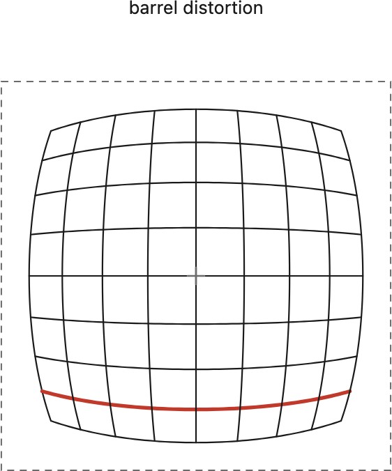
The symptom is bowed lines. A real lens images world-straight lines as gentle curves. In barrel distortion the lines bow outward and the frame seems to fatten (magnification falls with radius), the signature of wide-angle lenses; in pincushion distortion they bow inward as magnification rises with radius, typical of telephoto; a blend of the two is mustache distortion. The radial model is symmetric about a fitted distortion center, often close to the principal point and worst at the edges, and its extreme case is the fisheye, where the bending is so strong it is no longer a defect to remove but the intended projection.
The model is a per-radius remap. Because the effect is radially symmetric, the correction is a one-dimensional function of radius $r$ (the distance from the optical center) applied along each ray: points move only in or out, never sideways. The two parametric forms are exactly the ones introduced in Chapter 22.1, Aberrations and optical challenges, used here in reverse. The polynomial (Brown–Conrady) model writes the distorted radius forward as
with $k_1<0$ for barrel and $k_1>0$ for pincushion; mapping a measured distorted point back to an undistorted point requires inversion. Rendering a corrected image usually needs the displayed forward map instead: for each undistorted output location, evaluate its distorted source location. One or two terms suffice for most lenses. The division (Fitzgibbon) model uses a rational form,
which captures strong wide-angle and fisheye distortion with fewer parameters and inverts more cleanly, which is why it is favored for calibration.
Where the parameters come from. Two routes. The first is a lens profile: a precomputed table of coefficients per (lens, focal length, aperture), shipped by Lightroom / Adobe Camera Raw, PTLens, or DxO and looked up automatically from the EXIF tags that name the lens; this is the very profile the lens-profile-correction pass above already plays back to undo vignetting and lateral CA, so distortion comes off in the same step. The second is to estimate the coefficients from the image itself by plumb-line calibration: find features that ought to be straight (a building edge, a horizon) and choose the $k_i$ or $\lambda$ that make the imaged lines straight, minimizing their residual curvature.
Applying it is an inverse warp. Once the radial map is known, it is applied by the same engine as every geometric resampling operation, inverse-warp and resample: loop over output pixels, push each back through the radial map to its source radius, and resample the input (the warping machinery developed in Chapter 11.1, Warping in the motion-and-video part, which now points back here for this lens correction). The stretched and compressed edge regions carry the usual prefilter-before-downsample care, and the corners that read past the frame are handled by the boundary policy or simply cropped. The correction can straighten lines accurately, but stretching cannot create the additional samples a corner would have received from an optically rectilinear lens. Use a suitable interpolant and account for the output crop.
22.2.5 Aberration data in the DNG, and the limits of per-copy correction⧉
The profile a raw converter plays back need not come from a separate database; increasingly it rides inside the file. A DNG can carry lens corrections as opcodes, small typed operations the standard defines and stages along the demosaic pipeline (the OpcodeList1/2/3 fields). The geometric ones are exactly the corrections above: WarpRectilinear encodes the distortion and lateral-chromatic-aberration polynomials as per-channel radial coefficients, FixVignetteRadial carries the vignetting gain, and WarpFisheye handles the fisheye map; beside them sit FixBadPixelsConstant/List for dead and hot pixels (the subject of Chapter 8.9, Dead pixels) and per-pixel gain maps. A camera or raw converter can write these opcodes when it has an appropriate calibration. Their presence, version, optional/required flags, and reader support determine which corrections travel with a particular file; not every DNG includes a complete lens profile. The DNG is self-describing: the correction travels with the pixels.
The catch is that a supplied correction may represent the lens model rather than the copy in your hand; the format itself does not forbid per-unit calibration, and real lenses do not leave the factory identical. A purely radial profile assumes rotational symmetry; more general calibration can include a shifted center, tangential terms, or spatial gain maps, but manufacturing tolerances break that assumption. Decentering, an element tilted or shifted by microns, makes the blur and even the distortion asymmetric, worse on one side of the frame than the other, which no centered radial map can remove. Sample variation means two copies of the same lens distort and vignette by slightly different amounts, and the profile splits the difference. And the errors drift with focus distance and, on a zoom, with focal length, so a profile indexed only by the nominal settings is always a little off. Lens-profile correction is therefore excellent at the designed defect and merely approximate for your lens: it straightens the nominal barrel but can leave a faint residual mustache, evens the nominal vignette but not a decentered one. Closing that last gap needs a per-copy calibration, which a few high-end workflows and cameras actually perform, measuring the individual lens rather than trusting the model average.