18.3 Two-scale and bilateral tone mapping🔗⧉

When the range is high, a global curve cannot compress it and keep local contrast at the same time (Chapter 18.2, Global tone mapping). Two-scale methods separate the two jobs. They split the image into a base layer, which carries the large-scale variations and most of the dynamic range, and a detail layer, which carries local contrast and texture; they compress the base and keep the detail. The idea matches what perception allows (Chapter 18.1, Tone mapping and perception): large-scale variations are mostly illumination, which the eye discounts, and local contrast is mostly reflectance, which it reads. This is also the reasoning of Land's Retinex theory of lightness, which estimates the illumination as a smooth version of the image in log space and attributes the rest to the surfaces Land & McCann 1971; its multiscale version was used directly to compress the range of photographs Jobson, Rahman & Woodell 1997 (multiscale Retinex). Everything depends on how the base is computed, and the history of the method is the history of that one choice. The filters themselves are developed in Part 10, Edges matter; this chapter covers their use for tone mapping and the failures they do and do not fix.

18.3.1 Starting with global tone mapping🔗⧉

We start with a simple global tone mapping approach based on a gamma remapping expressed in log values. High-dynamic-range tone mapping is a task where the choice of encoding really matters (Chapter 4.3, Encoding: linear, gamma or log). Working in log luminance, where ratios become differences (Chapter 18.2, Global tone mapping), was recognized decades ago with so-called homomorphic filtering Oppenheim, Schafer & Stockham 1968 (homomorphic filtering), which suggests that when dealing with phenomena that involve multiplications (such as the product of reflectance and illumination), one should work on log values. Log conforms to the visual system's relative invariance to multiplication factors. Any base works, and Durand and Dorsey, like the figures here, use $\log_{10}$. With $Y$ the luminance of the radiance map,

In log values, the multiplicative dynamic range $Y_{\min}:Y_{\max}$ becomes a simple additive range $\log Y_{\max}-\log Y_{\min}$ (Figure 18.3.1⛶ fullscreen, stage input). We can map it to the limited dynamic range of a display (or a target set by the user) $1:\mathrm{DR}$ with a gamma remapping curve (not to be confused with gamma encoding, Chapter 4.3, Encoding: linear, gamma or log; the two are related by the system gamma), with exponent $c$ given by the ratio of output and input dynamic range in log. The gamma exponent becomes a multiplication in log:

Subtracting $\log Y_{\max}$ sends the brightest pixel to $\ell_\text{out}=0$, that is to display white, and the darkest to $-\log\mathrm{DR}$. For a scene of 1:10,000 shown on a display of 1:100, $c=2/4=0.5$.

If we apply this curve to $R$, $G$ and $B$ separately, the colors wash out (Figure 18.3.1⛶ fullscreen, stage per-channel). The exponent pulls every ratio toward one, including the ratios between the channels: a saturated red with $R/G=4$ comes out with $R/G=4^{0.5}=2$ for $c=0.5$, much closer to gray. Chroma and saturation are carried by these ratios, so to preserve them we apply the curve to the luminance alone and put the color back by keeping each pixel's ratios $R/Y$, $G/Y$ and $B/Y$:

The ratios do not change when a pixel is made brighter or darker, which is why they can be held fixed while the luminance is compressed. All of these are linear values; the output still needs the display encoding. Keeping the ratios exactly is a starting point rather than a law of perception, and Chapter 18.2, Global tone mapping discusses its limits and the alternatives.

The colors are now right, but the image looks flat and muddy (Figure 18.3.1⛶ fullscreen, stage luminance). The curve reduces every ratio by the same exponent, small ones as well as large ones: with $c=0.5$ the ratio between the window and the room drops from 10,000 to 100, as intended, and the 2:1 contrast of a texture or of the shading on a face drops to $2^{0.5}\approx1.4$:1. Reducing contrast was the job of the curve, so a global curve cannot avoid it; it cannot tell the large ratios it must compress from the small ones we would like to keep.

18.3.2 Base and detail🔗⧉

The idea of two-scale tone mapping is to apply the gamma contraction only to a large-scale layer of the image, which holds most of the range, and to leave the small-scale variations, which hold the local contrast, untouched. The same idea can be reached from different perspectives. The large-scale layer tells us if a region of an image is bright or dark and we seek to darken bright regions and vice versa, similar to dodging and burning in the darkroom (Chapter 5.5, Developing and editing a photograph; Chapter 18.9, High dynamic range in traditional photography). Or we can view the base as trying to estimate illumination while the detail represents reflectance or albedo variation, and given the human visual system's focus on reflectance, and the limited dynamic range of reflectance, we can afford to compress the contrast of the illumination.

We first attempt to create a base or large-scale layer $B$ using a simple Gaussian blur on the log luminance. The detail $D$ is simply the difference between the original log luminance and the base.

with $G_{\sigma_s}$ a Gaussian of width $\sigma_s$; the methods of the following sections change only this filter. We compress the base with the exponent $c$ and add the detail back unchanged, or amplified by a factor $a$:

The factor $c$ is the exponent of the global curve, now applied to the base alone. We choose it so that the base fits the target output contrast: if the base spans $\Delta B=B_{\max}-B_{\min}$ in log units and the display should show a contrast of $1:\mathrm{DR}$, then $c=\log\mathrm{DR}/\Delta B$. As in the global curve, subtracting $B_{\max}$ puts the brightest part of the base at white; a high percentile is a more robust choice, as in the bilateral method below. With $a=1$ the detail keeps exactly the local contrast it had in the scene; $a>1$ exaggerates it. Color is put back with each pixel's color ratios, as in the global curve.

two_scale_tonemap(Y, rgb, DR, sigma_s, detail_amp=1):
    l = log10(max(Y, eps))
    B = gaussian_blur(l, sigma_s)         # the following sections change only this line
    D = l - B
    c = log10(DR) / (max(B) - min(B))
    l_out = c * (B - max(B)) + detail_amp * D      # brightest base value at 0, i.e. white
    Y_out = 10 ** l_out
    return rgb * (Y_out / Y)[..., None]   # then exposure, gamma or display encoding

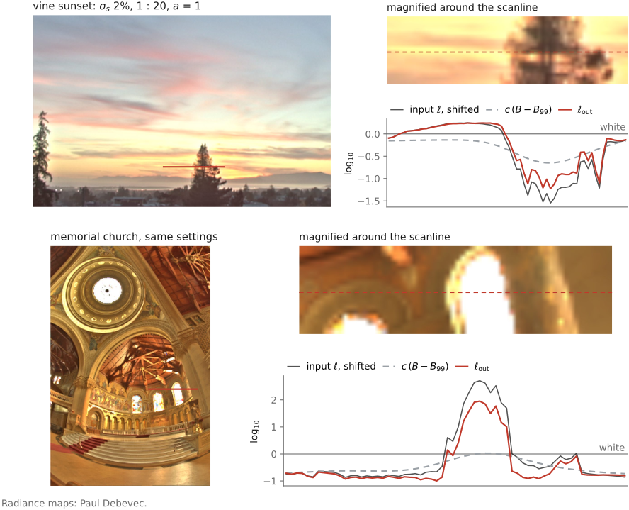
With the Gaussian base, smooth regions come out well: the blur averages away the detail and keeps the slow variations, and compressing it leaves the texture intact. The trouble is strong edges. A Gaussian blur does not respect edges: it averages straight across the boundary between the bright window and the dark wall, so near that edge the base is a smeared ramp, too dark on the bright side and too light on the dark side. When we compress this base and add the detail back, the error shows. With $a=1$ the output is $\ell_\text{out}=\ell-(1-c)\,B$ up to a constant, so where the base is too low, on the bright side, too little is subtracted, and where it is too high, on the dark side, too much: next to the edge the bright side comes out brighter still and the dark side darker, a band on each side that exaggerates the edge. This is a halo (Figure 18.3.2⛶ fullscreen; Figure 18.3.1⛶ fullscreen, stage gaussian, follows it on a profile across an edge). It is the same failure mode as naive unsharp masking, and it is the signature artifact of cheap local tone mapping, the glow around the skyline in an over-processed HDR photograph.

This first attempt has a history. Homomorphic filtering, met above, already reduced the slowly varying illumination of the log image with a low-pass filter while keeping the reflectance. The first tone-mapping operator of this kind is Chiu and colleagues' of 1993, and its failure is the most instructive one in this area Chiu et al. 1993. They scaled each pixel by the inverse of a heavily blurred copy of the image, which compresses large-scale variations and keeps the small ones. Where the scene is smooth it works. At a strong edge the blur mixes both sides, and the result is a wide band of false brightness along every high-contrast boundary. The fifteen years of research that followed were mostly about how to compute the large-scale layer without that mixing, rather than about the tone curve applied to it.

An edge-preserving filter reduces mixing across strong boundaries. Its range weights can greatly reduce halos, but do not guarantee their absence; parameter choice, noise, and subsequent clipping still matter. Part 10, Edges matter develops the filtering machinery. Even then, a base/detail decomposition is an approximation, not a unique description of the scene. Large illumination differences often enter the base, while texture and noise enter the residual. Compressing only the base preserves the residual numerically; it does not establish that every preserved variation is useful detail.

18.3.3 LCIS: diffusion that stops at edges🔗⧉

The fix for the halos is a smoothing that does not cross strong edges. Tumblin and Turk's low-curvature image simplifiers, LCIS, were the first tone-mapping operator to do this deliberately Tumblin & Turk 1999 (LCIS). Their starting point was the way an artist sketches a scene: large regions with sharp boundaries, filled with smooth shading, with the detail added on top. LCIS is a form of anisotropic diffusion (Chapter 10.1, Bilateral filtering): it repeatedly smooths the image within regions and stops at boundaries where the curvature of the intensity is high, so a strong edge survives while the shading on either side flattens. Run for increasing times, it produces a hierarchy of simplified images, each a candidate base layer, and the detail is the difference between successive levels. Compressing the most simplified level and adding the details back removed most of the halos of the blurred base. The method was slow, since the diffusion takes many iterations, and it could leave its own artifacts, thin bright or dark lines along strong edges where the diffusion stopped abruptly.

18.3.4 Bilateral tone mapping🔗⧉

Durand and Dorsey replaced the diffusion with the bilateral filter, which computes an edge-preserving base in one pass Durand & Dorsey 2002. The bilateral filter averages each pixel with neighbors that are both close in space and close in value (Chapter 10.1, Bilateral filtering). For the log intensity $\ell$, at pixel $p$,

with $f$ a Gaussian of width $\sigma_s$ in space and $g$ a Gaussian of width $\sigma_r$ in log intensity. Near a strong edge the pixels on the far side differ by much more than $\sigma_r$, their range weight is nearly zero, and the average stays on its own side: the base keeps the edge sharp, and the detail layer, the difference between the image and its base, contains no trace of it. Working on log intensity is what makes this right for tone mapping. The range weight then compares ratios, so an edge is "strong" when its contrast is large, whatever the absolute brightness: a window ten times brighter than a wall is excluded from the wall's average in the shadows and in the highlights alike. Since the eye also responds to ratios, the filter's notion of an edge matches the viewer's.

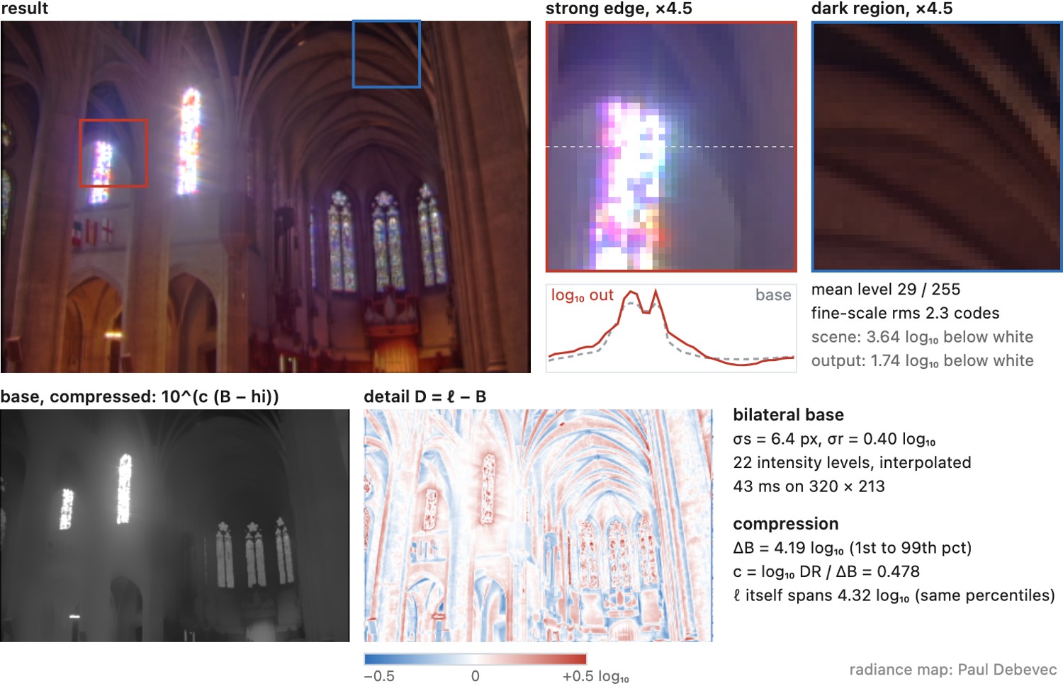
Figure 18.3.3⛶ fullscreen shows the two layers a bilateral base gives on a real scene.

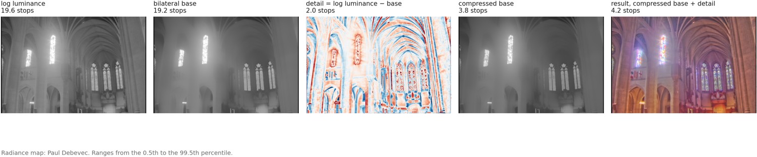
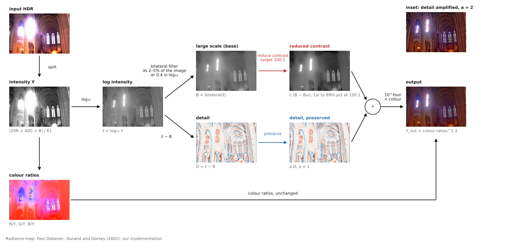
The whole operator follows the diagram of Figure 18.3.4⛶ fullscreen, in six steps.

1. Separate intensity and color. Compute an intensity from the radiance map, a weighted sum of the channels; the paper used $Y=(20R+40G+B)/61$, and any luminance will do. Divide the channels by it to get the color ratios $R/Y$, $G/Y$, $B/Y$, which carry the color independently of the brightness. This is the separation of luminance and color met above with the global curve, and for the same reason: compressing $R$, $G$ and $B$ separately would wash out the colors.
2. Take the logarithm of the intensity, $\ell=\log_{10}Y$.
3. Compute the base with the bilateral filter, $B=\mathrm{bilateral}(\ell)$. Typical parameters are a spatial width $\sigma_s$ of 2 to 5% of the image size, and a range width $\sigma_r$ of 0.4 in $\log_{10}$, a factor of about 2.5 in intensity.
4. Compute the detail, the residual $D=\ell-B$.
5. Compress the base. Choose the contrast $1:\mathrm{DR}$ the base should have on the display, for instance 1:100. The base spans $B_{\max}-B_{\min}$ in log units, so the compression factor is $c=\log_{10}\mathrm{DR}/(B_{\max}-B_{\min})$. The output log intensity is

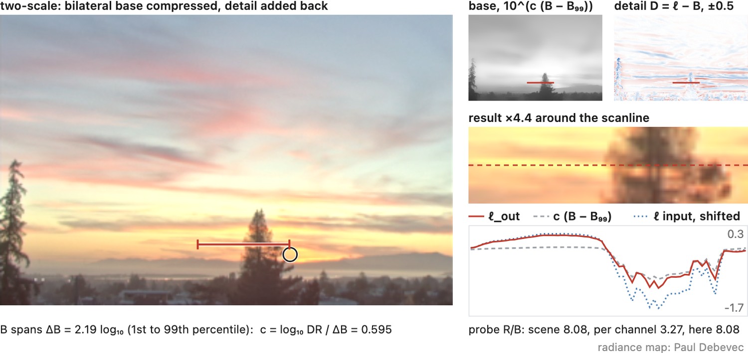
where subtracting $B_{\max}$ puts the brightest part of the base at zero, that is at white, and $a$ is the detail amplification, one to keep the detail as it was. In practice the extremes are better taken as percentiles, the 1st and 99th for instance, so that a few hot pixels or specular points do not set the scale for the whole image, as Figure 18.3.4⛶ fullscreen and the explorer of the next section do.

1. Recombine. $Y_{\rm out}=10^{\ell_{\rm out}}$, and each channel is $Y_{\rm out}$ times its color ratio. The result is display-linear and still needs the output encoding.

bilateral_tonemap(R, G, B, sigma_s=0.02*width, sigma_r=0.4, DR=100, detail_amp=1):
    Y = (20*R + 40*G + B) / 61                    # intensity
    r, g, b = R/Y, G/Y, B/Y                        # color ratios, independent of brightness
    L = log10(Y)
    base = bilateral(L, sigma_s, sigma_r)          # edge-preserving large scale
    detail = L - base                              # residual: texture and local contrast
    hi, lo = percentile(base, 99), percentile(base, 1)   # robust max and min
    c = log10(DR) / (hi - lo)                      # compress the base to the target contrast 1:DR
    L_out = c * (base - hi) + detail_amp * detail  # bright end of the base at 0, i.e. white
    Y_out = 10 ** L_out
    return Y_out*r, Y_out*g, Y_out*b               # then gamma or the display's encoding

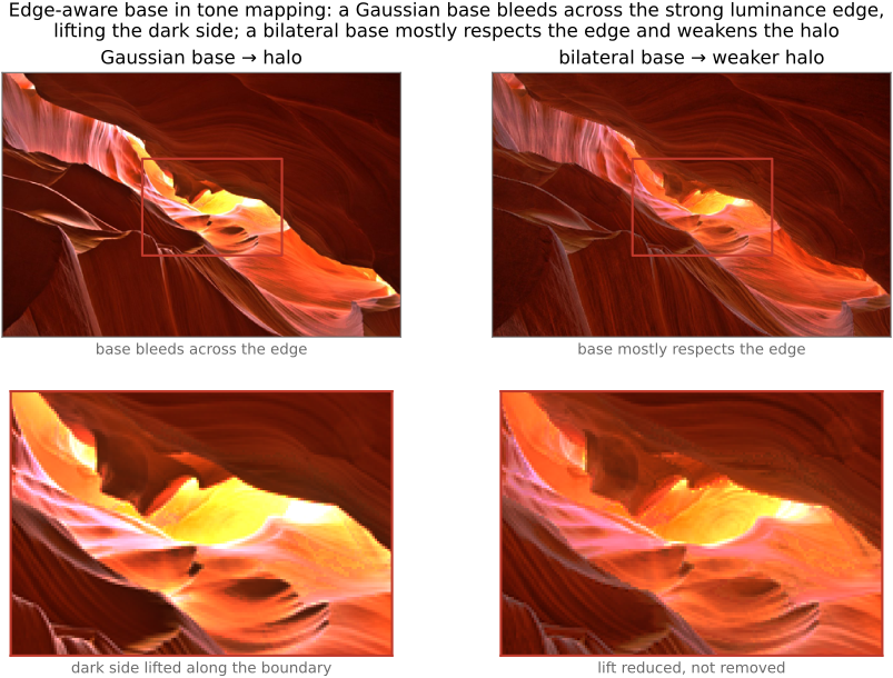
On the sunset, the bilateral base removes the halo of the Gaussian one (Figure 18.3.1⛶ fullscreen, stage bilateral).

What matters. The method has few parameters, and they do not matter equally. The spatial width $\sigma_s$ is not critical: anything from about 2 to 5% of the image size gives similar results, because it only has to be larger than the texture and smaller than the regions. The range width $\sigma_r$ matters much more. Too small, and moderate texture counts as edges, so it stays in the base and is compressed; too large, and strong edges are averaged across, and the halos of the Gaussian base return. The log domain is essential, for the two reasons above: the scene's range is too large for a range weight on linear values to make sense, and contrast is perceived as a ratio. The choice of intensity is less critical but changes the result; a better function of the channels can help, as in the flash and no-flash work that followed Eisemann & Durand 2004. Figure 18.3.6⛶ fullscreen, in the next section, lets the reader vary both widths.

Detail amplification. With $a>1$, the detail layer is amplified: textures and small contrasts become more pronounced than in the scene. In moderation this restores the local contrast that viewers expect from a print; pushed far, it produces the overprocessed look discussed below.

A single image. The operator does not need a bracket. A raw file from a modern camera holds 12 to 14 stops (Chapter 17.1, Dynamic range and multiple-exposure capture), more than a display shows, and benefits from the same compression; shadow-lifting tools in raw developers are close relatives. The limit is noise: lifting the base of a dark region raises its noise along with its detail, since the detail layer contains both.

Speed. Computed directly, the bilateral filter is slow: each pixel averages a large neighborhood with weights that depend on the pixel itself, so it cannot be done as a convolution, and on the images of 2002 a direct implementation took minutes. Durand and Dorsey made it fast by linearizing it. They chose a small set of intensity levels; for each level, the range weight is a fixed function of the pixel values, so the weighted sums $\sum_q f\,g\,\ell_q$ and $\sum_q f\,g$ become ordinary convolutions, computed with fast Fourier transforms and at reduced resolution; each pixel then interpolates the result between the two levels nearest its own intensity. This piecewise-linear acceleration was the first step toward the bilateral grid, which treats intensity as a third dimension, splats the image into a coarse three-dimensional grid, blurs it and reads it back, and runs in real time on a graphics processor Paris & Durand 2009 Chen et al. 2007 (Chapter 10.1, Bilateral filtering).

18.3.5 The decomposition zoo, and what it fixes🔗⧉

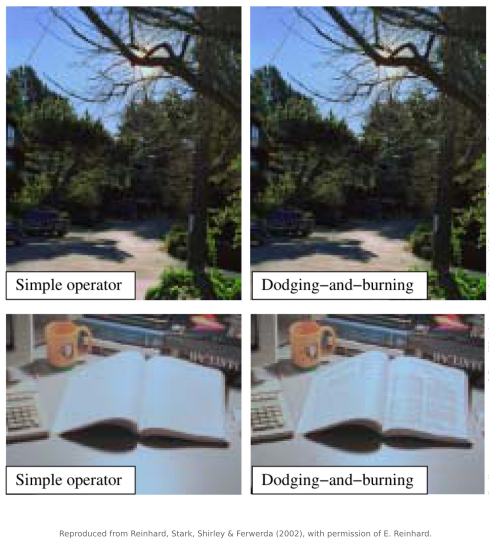
Reinhard and colleagues reached an edge-aware base from the darkroom side. Their automatic dodging-and-burning chooses, at each pixel, the largest neighborhood over which the image is roughly uniform, by comparing blurs at successive scales and stopping before one straddles a strong edge, and uses that neighborhood's average as the local adaptation level Reinhard et al. 2002. The per-pixel scale selection is an edge-aware base by another route.

After the bilateral filter, many edge-preserving smoothings were proposed as better bases, each developed in Part 10, Edges matter. The weighted-least-squares smoothing of Farbman and colleagues solves for a base that stays close to the image while being smooth except where the image gradient is large, and supports a multiscale split into several detail layers; at a large spatial scale it lets a bright window's glow return Farbman et al. 2008. The guided filter computes a locally linear fit to a guide image and is fast and free of the bilateral's gradient reversals, though it softens a strong step slightly, by about a tenth in the explorer below He, Sun & Tang 2013 (guided filter) (Chapter 10.6, Guided image filtering). The bilateral grid makes the bilateral real-time on a graphics processor Chen et al. 2007, and HDRnet learns to predict local affine tone adjustments in such a grid from examples (Chapter 18.8, Display rendering transforms and color).

They differ in what they fix. Edge-aware bases greatly reduce halos at strong edges, but none removes them everywhere: an edge with a moderate contrast, close to the filter's range scale, is partly smoothed, and a soft halo remains. The bilateral filter can produce gradient reversals, thin bright or dark lines along edges that a smooth ramp should have crossed, because it treats a pixel on a ramp as an outlier; the weighted-least-squares and guided filters reduce them. None of them fixes noise. The detail layer contains the sensor noise along with the texture, and when the base of a dark region is raised while its detail is kept, the noise there is raised in relative terms; denoising before tone mapping, or limiting detail gain in dark regions, is part of a working pipeline. And none fixes the look. A detail gain above one, or a base compressed too far, flattens the large-scale relationships of the scene, the dark sky that ends up as bright as the lit facade, which is the overprocessed look of many HDR photographs of the 2000s. That is a choice of parameters, not a failure of the filter.

Figure 18.3.6⛶ fullscreen puts the four bases side by side on one radiance map, with the halo and the noise each under a magnifier.