6.3 Fourier⧉
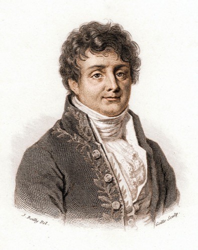 Joseph Fourier (1768–1830) reached his transform not through pure mathematics but through physics: the conduction of heat. In the 1822 Théorie analytique de la chaleur he made the then-scandalous claim that any function, however jagged, can be written as a sum of sines and cosines; contemporaries including Lagrange doubted it, and pinning down exactly when it holds occupied analysts for a century after. The decomposition into frequencies that diagonalizes convolution (the engine of this whole chapter) is his. (Fourier also argued that the atmosphere keeps the Earth warmer than incoming sunlight alone would: the first description of what we now call the greenhouse effect. He was, briefly, Napoleon's governor of Lower Egypt, too.) Portrait: engraving after Julien-Léopold Boilly, early 19th c., public domain (via Wikimedia Commons).
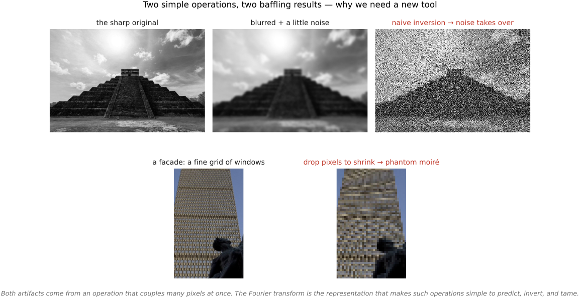
Fourier analysis rests on a change of representation: treat an image or signal as a sum of sine waves instead of a grid of pixels. It lets us answer rigorously the questions the previous chapters raised, and see what is possible, hard, or impossible. Start with two simple operations (Figure 6.3.1). First, deblurring: take a blurry photo for which we know the linear blur process but where noise further degrades the image. Try to undo the blur with direct linear inversion. Instead of the sharp original, the result explodes into noise. Second, downsampling: shrink a photo of a building facade by simply keeping every seventh pixel, and bold curved bands appear that are nowhere in the building: phantom moiré. Neither result is a bug; both are doing exactly what we asked. What makes them so hard to reason about is that each operation couples a great many pixels at once: a blur mixes every neighbor into every output, and decimation's fate depends on how the discarded pixels related to the kept ones across the whole image. Staring at the pixels tells us nothing. To understand how these artifacts and patterns emerge, and how to predict, invert, and tame them, we need a different mathematical tool, one in which these many-pixel operations become simple enough to analyze at a glance. That tool is the Fourier transform.
For the very same reason (that it captures blur so cleanly), Fourier is also the standard language for evaluating imaging systems. Because a lens or sensor blurs by convolving with its point-spread function, its contrast transfer can be described locally in the frequency domain by a modulation transfer function (MTF): how much contrast survives at each spatial frequency. MTF curves are how optics are actually specified and resolution is measured (a section below returns to this), so the machinery we build here to fight blur is the same machinery the industry uses to measure it. The eye works this way too: its own sensitivity to detail is a function of spatial frequency, the contrast sensitivity function (CSF) of Chapter 3.4, Spatial and temporal vision, so the frequency picture matches how we see as well as how lenses blur.
Fourier also describes wave propagation. In a suitable coherent optical setup, a lens maps the input field amplitude to its Fourier transform in a focal plane. A detector measures the squared magnitude of that field. This distinction matters when using Fourier to explain diffraction.

Fourier is useful even when we never compute a spectrum. It explains why blur is difficult to invert and why sampling creates aliases. It also supplies practical algorithms: FFT convolution, frequency-domain deconvolution, and transform coding. JPEG uses a related cosine transform (Chapter 8.11, File formats and compression).
A finite DFT represents a periodic signal. Padding lets an FFT compute ordinary finite convolution exactly; failing to pad instead computes circular convolution. We distinguish these boundary choices below.
6.3.1 Why Fourier⧉
We saw in Chapter 6.2, Convolution that convolution is a linear operator, and a linear operator is just a matrix. Stack an image's pixels into one long vector $\mathbf{x}$, and a blur becomes a single large matrix $M$ that carries the sharp image to the blurred one, $\mathbf{y} = M\mathbf{x}$. Here is the catch. That matrix is enormous, and painful to reason about and, above all, to invert: undoing the blur means untangling all the overlapping neighborhoods at once, and a clean, local operation can have a thoroughly non-local undo. You cannot eyeball a million-by-million matrix and pronounce whether it can be undone. For zero-extended one-dimensional convolution, the matrix is Toeplitz, the same kernel sliding down every row, constant along each diagonal, clean enough to draw. In 2-D that tidiness fragments: once you flatten the grid into a vector, the matrix becomes a block-of-Toeplitz-blocks, far messier to picture even though it is doing the very same local averaging. That is one more reason to change basis rather than wrestle the matrix directly.
There is, however, one species of matrix that is trivial to understand and trivial to invert: a diagonal matrix. A diagonal matrix has no cross-talk: each input coordinate is multiplied by its own scalar, independently of every other. Inverting it is then trivial: divide each coordinate by that scalar. The entire difficulty of inversion shrinks to one question per coordinate: how close is that scalar to zero? Dividing by a near-zero number is where all the trouble lives.
So the goal is clear: we would love the blur matrix to be diagonal. In the pixel representation it is nowhere close. But, and this is the pivot of the chapter, we are free to change how we represent the image, to describe it in a different basis, and a linear operator that looks coupled and hard to invert in one basis can look perfectly diagonal in another. The basis that diagonalizes convolution is precisely the Fourier transform. Change to the Fourier representation and blur stops being a million-dimensional tangle and becomes, instead, a separate scalar multiplication on each frequency, exactly the diagonal case we wished for. (For finite arrays, the DFT diagonalizes circular convolution. An ordinary finite convolution can be embedded in a larger circular one by padding, as the implementation below shows.)
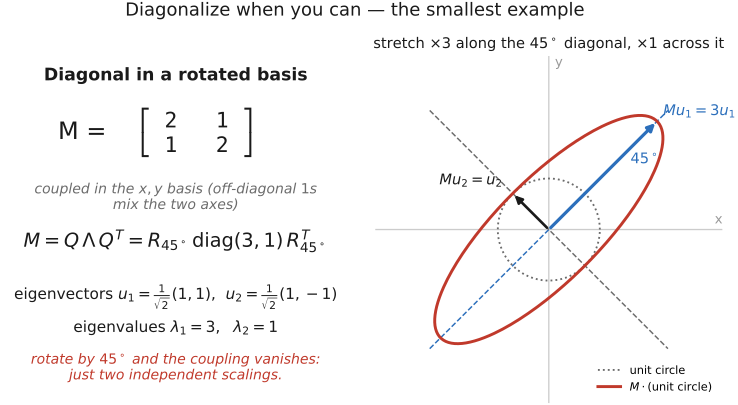
Express a linear operator in a basis where it becomes diagonal. A coupled, hard-to-invert operation in one representation can be a list of independent scalar multiplications in another, and scalars are trivial to understand, compose, and invert. Fourier diagonalizes convolution, turning a blur into per-frequency multiplication. This is not a one-off trick: it is the single most reusable move in applied linear algebra, and it returns for differential equations (the heat equation, below), for principal components, and for nearly every inverse problem in this book. The idea is already visible in the smallest possible case, a $2\times2$ matrix (Figure 6.3.3).
And there is a bonus that makes Fourier feel less like a computational convenience and more like the right language for images. We have already met spatial frequency once, back in perception: the contrast sensitivity function (CSF) describes the eye's sensitivity as a function of how fine or coarse a pattern is, its spatial frequency (see Chapter 3.4, Spatial and temporal vision). The visual system is, to a first approximation, organized by frequency. So the Fourier view matches both the mathematics of convolution and the structure of human vision, which is why frequency keeps reappearing: in JPEG compression, in image-quality metrics, in tone mapping. When two unrelated considerations point at the same representation, that representation is usually the one to learn.
6.3.2 Complex waves are eigenvectors of shifts and convolution⧉
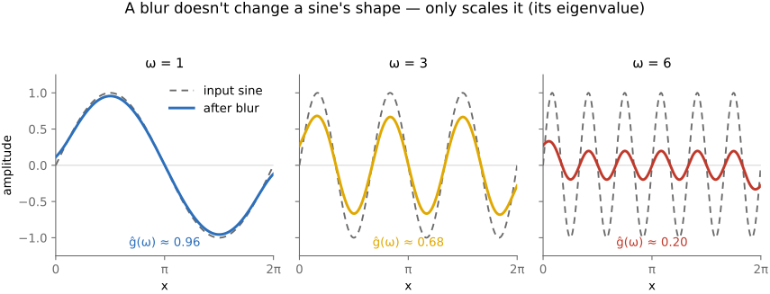
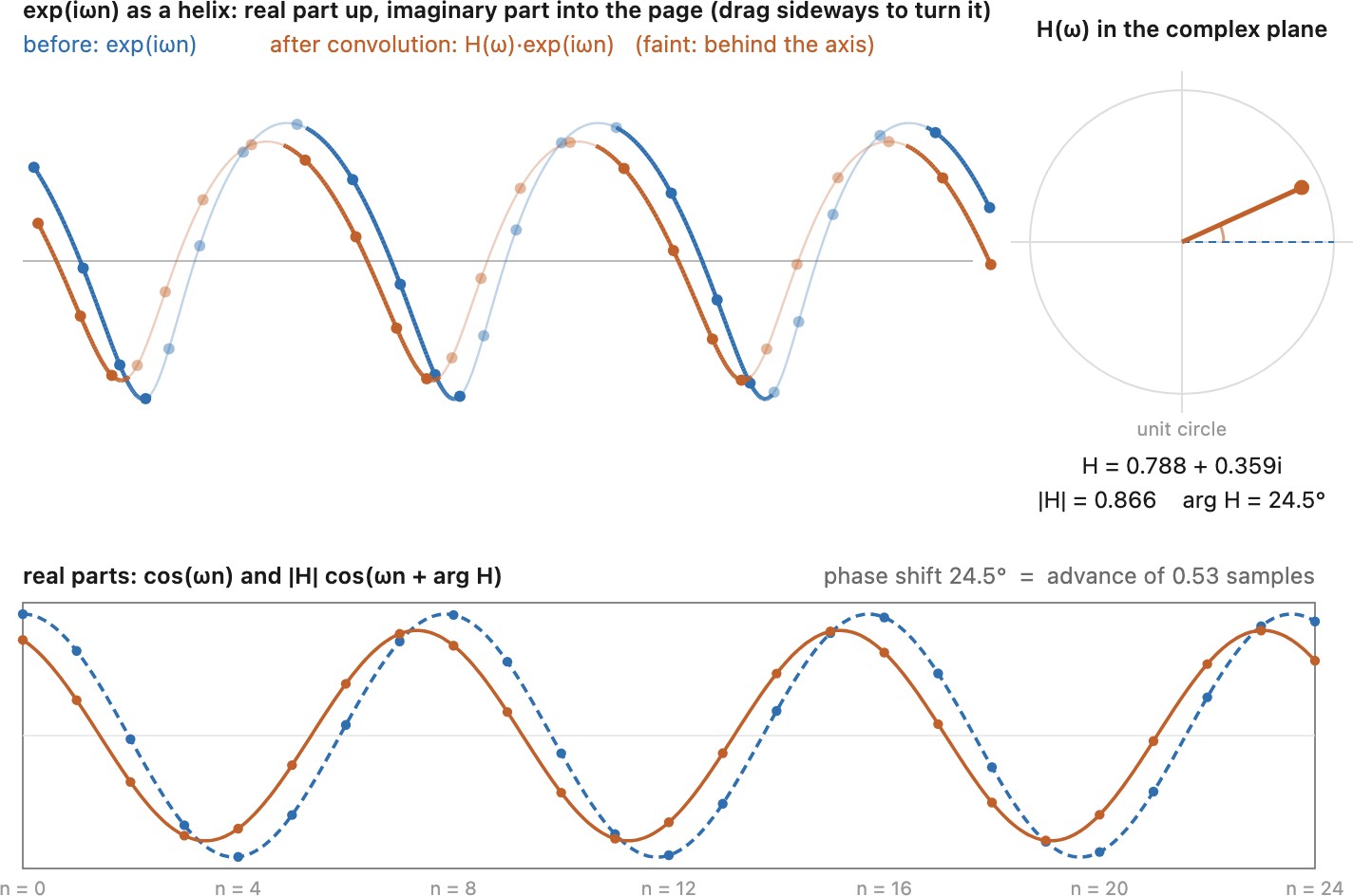
We have asserted that Fourier diagonalizes convolution. Here is the one-line reason, and it is the mechanical heart of the chapter. Start with the simplest operator of all, a plain shift. Slide a complex sine wave $e^{i\omega x}$ over by $d$ and you get $e^{i\omega(x - d)} = e^{-i\omega d}\,e^{i\omega x}$: the same wave at the same frequency, only multiplied by a constant phase $e^{-i\omega d}$. A complex exponential is therefore an eigenvector of translation, its frequency untouched and its eigenvalue a pure phase. Now recall that a convolution is nothing but a weighted sum of shifts (the sum-of-translated-images reading of the previous chapter). A weighted sum of shifts acting on our wave is a weighted sum of phases, still one number times the same wave, so a complex exponential is automatically an eigenvector of every convolution as well. Concretely, feed a pure sine wave into any convolution, any blur, and what comes out is the same sine wave, same frequency, only with its amplitude scaled and its phase possibly shifted (Figure 6.3.4). The wave is never bent into a different frequency; it is merely turned down (or up) and slid over. In the language of linear algebra, the complex exponentials are the eigenvectors of convolution, and the per-frequency scale factor is the eigenvalue. Symbolically, convolving a wave $e^{i\omega x}$ by a kernel $g$ just multiplies it by a number $\hat g(\omega)$ that depends only on the frequency:
A shift-invariant linear filter preserves frequency. Its complex gain can change amplitude and phase. A normalized smoothing kernel has gain one at DC and generally attenuates fine detail, but its response need not decrease monotonically: a box filter has zeros and side lobes. A real sinusoid stays sinusoidal; when its phase changes it is not, by itself, a real eigenvector.
Because every frequency is scaled independently, the whole convolution, written in the Fourier basis, is diagonal: the eigenvalues $\hat g(\omega)$ sit on the diagonal and nothing else. This is the convolution theorem, and it is the sentence to memorize:
Convolution in space is multiplication in frequency: transform the image and the kernel, multiply their spectra frequency by frequency, transform back. Everything else in this chapter is a consequence of that single identity.
Once you accept that a kernel's Fourier transform is its per-frequency gain, you can read a filter's entire behavior off the shape of $\hat g$, and conversely recognize a kernel from its spectrum. We gather the handful of kernels that recur most, and their spectra, alongside the other canonical transform pairs in the bestiary below.
6.3.3 The tiniest Fourier transform in the West⧉
A million dimensions is impossible to picture, so shrink the image to two pixels, a vector in the ordinary 2-D plane, with the two pixel values as its $x$ and $y$ coordinates (Figure 6.3.6). Take the simplest blur: each output pixel is $0.8$ of itself plus $0.2$ of its neighbor. As a matrix in the pixel basis this mixes the two coordinates: it is not diagonal; the off-diagonal $0.2$ is the cross-talk.
Now rotate the coordinate axes by 45°, onto the two directions $[1, 1]$ (both pixels equal, the constant, the zero-frequency or direct current (DC) term, borrowing the electrical-engineering name) and $[1, -1]$ (the two pixels opposite, the highest frequency a two-pixel image can carry). These two orthogonal axes give the normalized two-point Fourier transform. The displayed matrix includes a reflection, so it is an orthogonal change of coordinates rather than a pure rotation. And in these rotated axes the very same blur is diagonal: the constant direction $[1, 1]$ passes through untouched (a flat signal cannot be blurred, eigenvalue $1$), while the oscillating direction $[1, -1]$ is attenuated to $0.6$ (since $0.8 - 0.2 = 0.6$, the high frequency is damped). Two pixels, two frequencies, two independent scale factors: the entire apparatus of the chapter in a picture you could draw on a napkin. Everything that follows is this, scaled up to a million dimensions.
Written out, the change of basis and the blur it diagonalizes are just $2\times2$ numbers: the two-point DCT $B_2$ conjugates the blur $M$ into a diagonal of its eigenvalues.
The two rows of $B_2$ are the DC and the highest-frequency wave; conjugating by them turns the off-diagonal mixing into two independent gains, $1$ and $0.6$.
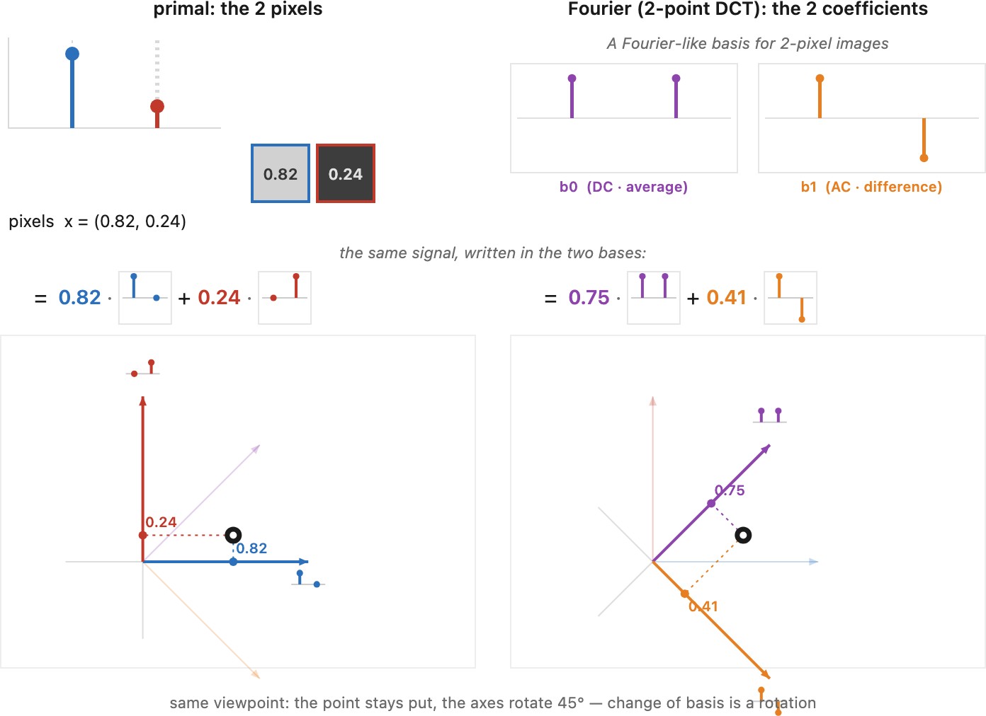
There are two ways to picture a change of basis, and they are worth holding apart: either the point stays fixed in space and the axes rotate around it, or you redraw both frames the same way and the point's coordinates move, transformed by the change-of-basis matrix. Same fact, two views; the 2-pixel figure above lets you toggle between them.
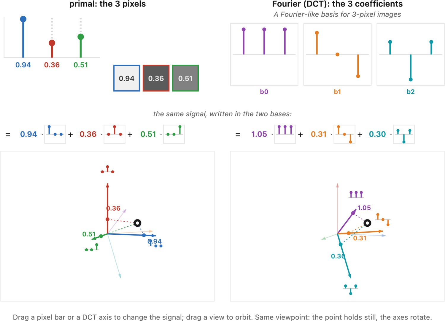
A three-pixel image is a point in 3-D. To keep this illustration real, we use the discrete cosine transform (DCT), whose axes here are a constant, a ramp, and a cosine (Figure 6.3.7). The DCT is related to Fourier analysis through an even extension of the signal. It is a different transform from the three-point DFT, whose nonconstant coefficients are complex.
Its matrix is again just numbers, the orthonormal three-point DCT, whose rows are the flat, ramp, and single-cosine waves.
The rows are orthonormal: lengths and angles are preserved, and the transpose gives the inverse. This matrix has determinant $-1$, so it includes a reflection.
6.3.4 Definition: one coefficient per wave⧉
Here is the transform itself, in words first. Instead of describing an image by one value per pixel, the Fourier transform describes it by one coefficient per sine wave. We fix a family of sinusoidal patterns, waves of every frequency that fit in the image, and ask, for each one, how much of that wave is present? The list of answers is the Fourier transform $\hat I$ of the image, and because the operation is perfectly reversible, that list carries exactly the same information as the original pixels: it is the same image, written in a different alphabet.
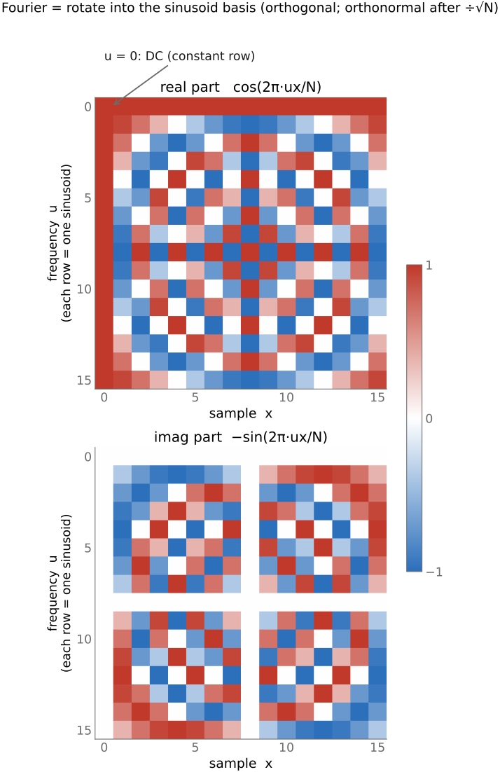
For an $N$-sample one-dimensional signal the recipe is a sum: one output coefficient $\hat I(u)$ for each frequency index $u$. This is the discrete Fourier transform (DFT):
Read it back in words: to find how much of frequency $u$ the signal holds, slide a wave of that frequency across the signal, multiply point by point, and add up, a dot product between the signal and that wave. The complex exponential $e^{-2\pi i\,ux/N}$ is just a compact way to carry a cosine and a sine of frequency $u$ together, by Euler's formula
so the real part of $\hat I(u)$ measures the cosine content and the imaginary part the negative of the sine projection. Why carry both? Because a single frequency can appear at any phase, shifted left or right, and a cosine and a sine of that frequency together can reproduce a wave of that frequency at any phase and amplitude. One pair, one cosine and one sine, per frequency. (The naive sum costs $O(N^2)$, but the fast Fourier transform (FFT) computes the very same coefficients in $O(N\log N)$, the algorithm that made Fourier methods practical, and the reason spectral tricks are cheap in code.)
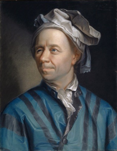 Leonhard Euler (1707–1783) was the most prolific mathematician who ever lived: he kept publishing for years after going blind, dictating from memory. The formula just above, $e^{i\theta}=\cos\theta+i\sin\theta$, is his, and it is what lets a single complex exponential carry a cosine and a sine together, the bookkeeping that makes the Fourier transform compact. His reach into this book is wide: the Euler–Lagrange equations we set to zero to minimize an energy (optical flow, Poisson blending), and the Eulerian "watch a fixed location" view of motion that names half of Chapter 12.4, Feature tracking and all of Chapter 38.3, Motion and video magnification. Portrait: by Jakob Emanuel Handmann, 1753, public domain (via Wikimedia Commons).
We use a negative exponent on the forward DFT and divide the inverse by the number of samples. Check the sign, normalization, and frequency units when translating formulas into code. A continuous transform, a Fourier series, and a finite DFT also describe different signal domains; they are not interchangeable definitions of the same array operation.

The waves are mutually orthogonal. With our unnormalized forward transform, each row of its matrix $F$ has norm $\sqrt N$, so $F^{-1}=F^*/N$, where $F^*$ is the conjugate transpose. Dividing both transform matrices by $\sqrt N$ gives the unitary convention used in geometric illustrations. The inverse of our DFT is
It adds the waves with their complex coefficients. The frequency index $u$ corresponds to $u/N$ cycles per sample, with indices above half the array interpreted as negative frequencies. In two dimensions the exponent becomes $-2\pi i(ux/W+vy/H)$, we sum over both pixel coordinates, and the inverse has factor $1/(WH)$.
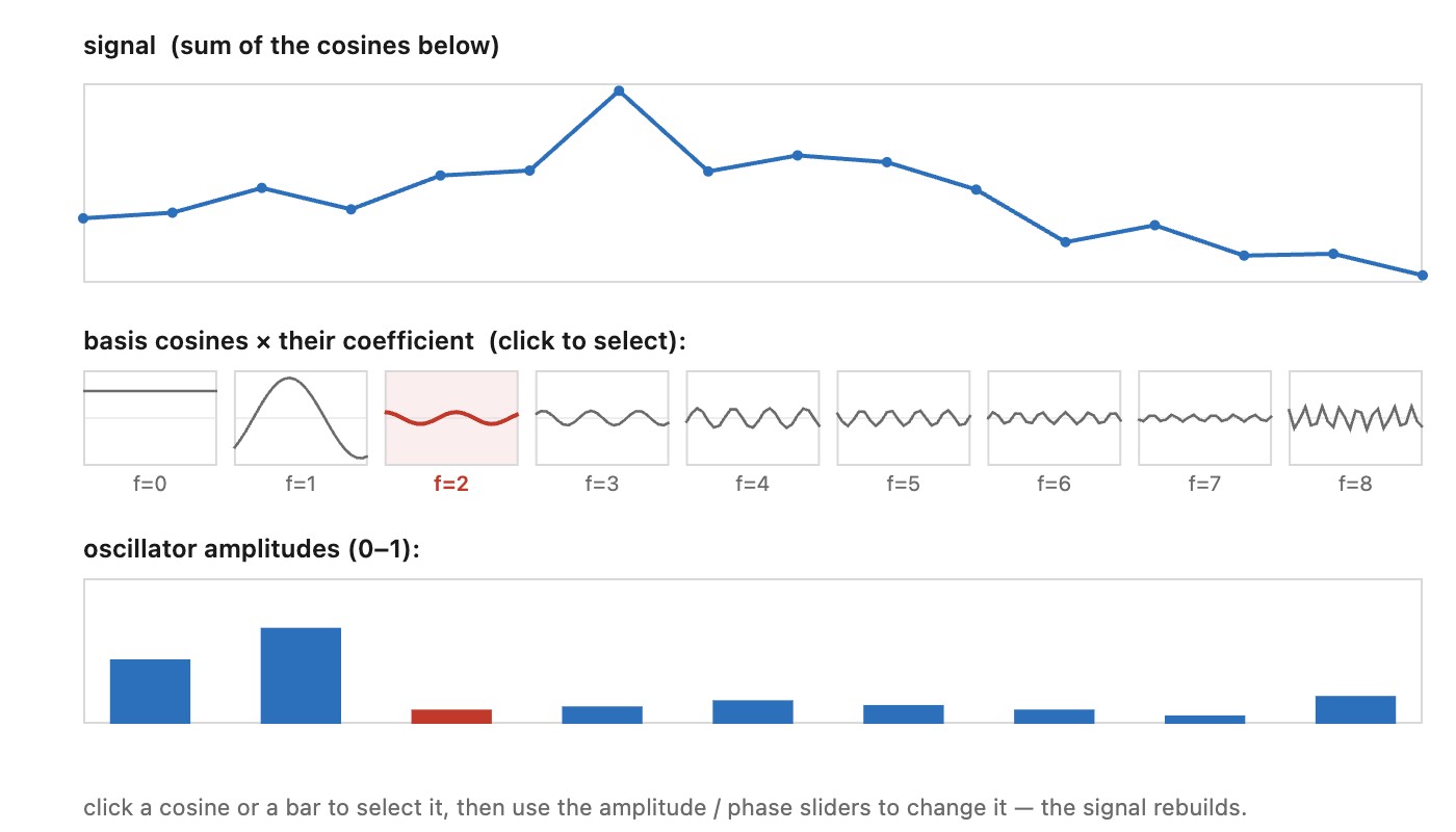
Read that inverse the other way and it becomes the most concrete statement of what the transform means: the signal is the sum of the basis waves, each weighted by its own coefficient. It is easiest to feel in one dimension first (Figure 6.3.10): a short signal is a sum of cosines, one per frequency, and adjusting a single wave's amplitude and phase reshapes the signal in the obvious way.
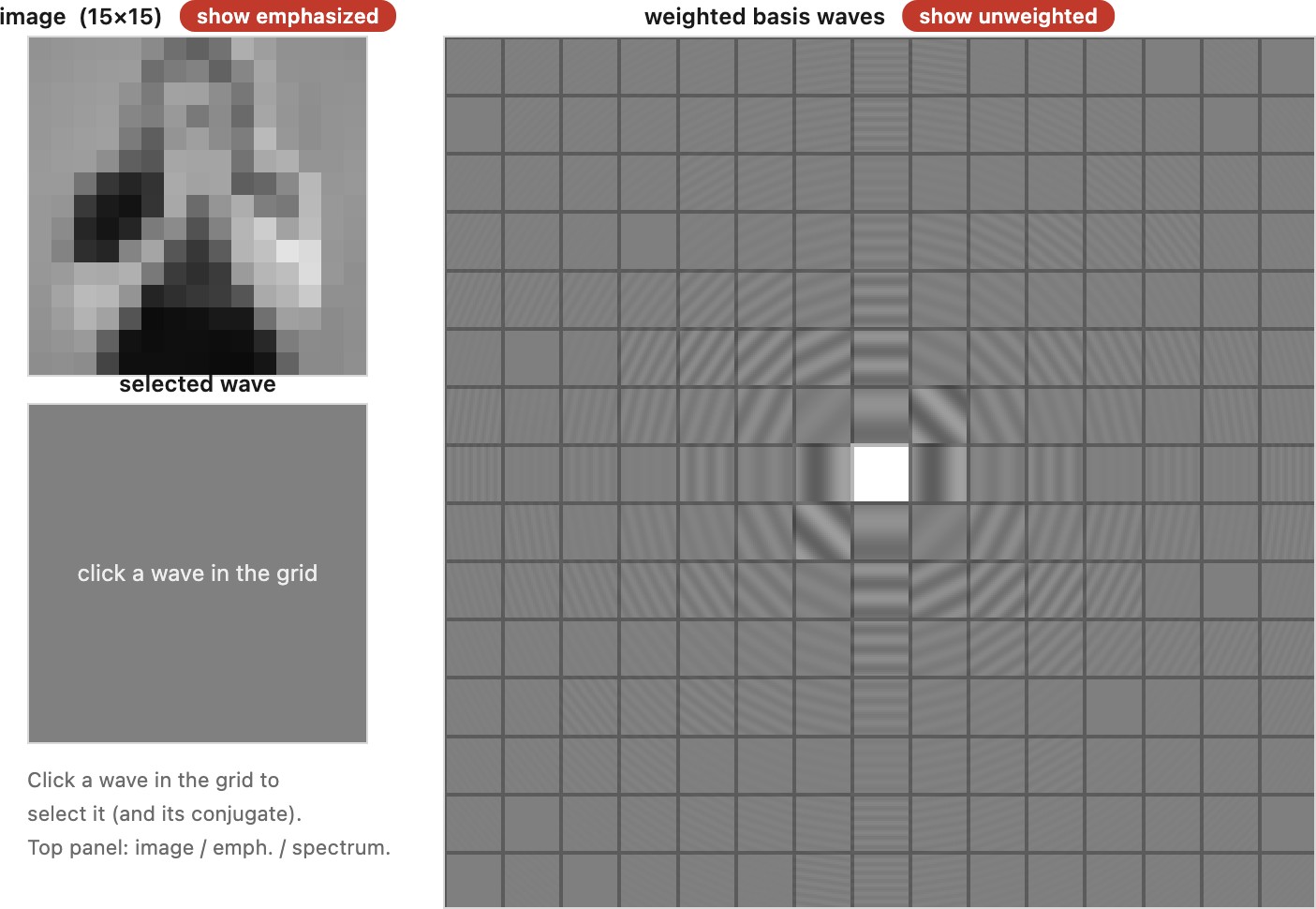
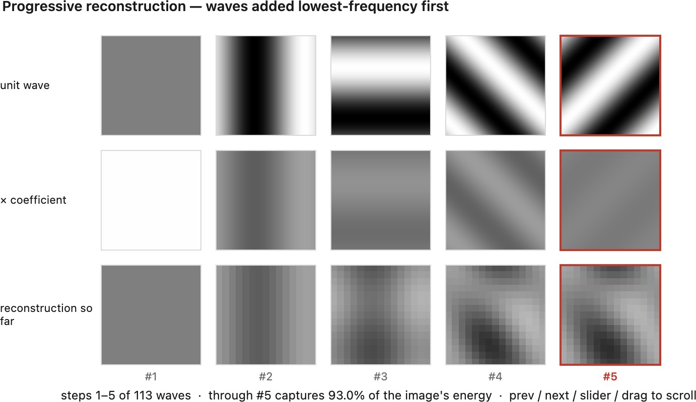
The same holds for an image, now with waves in two dimensions. Every picture, however busy, is a stack of plain 2-D sinusoids added together, and the Fourier transform is nothing more than the list of how much of each one to add. You can see this directly (Figure 6.3.11): dial the resolution down to a handful of waves, watch a recognizable image fall out of their sum, and click any single wave to see exactly what it contributes.
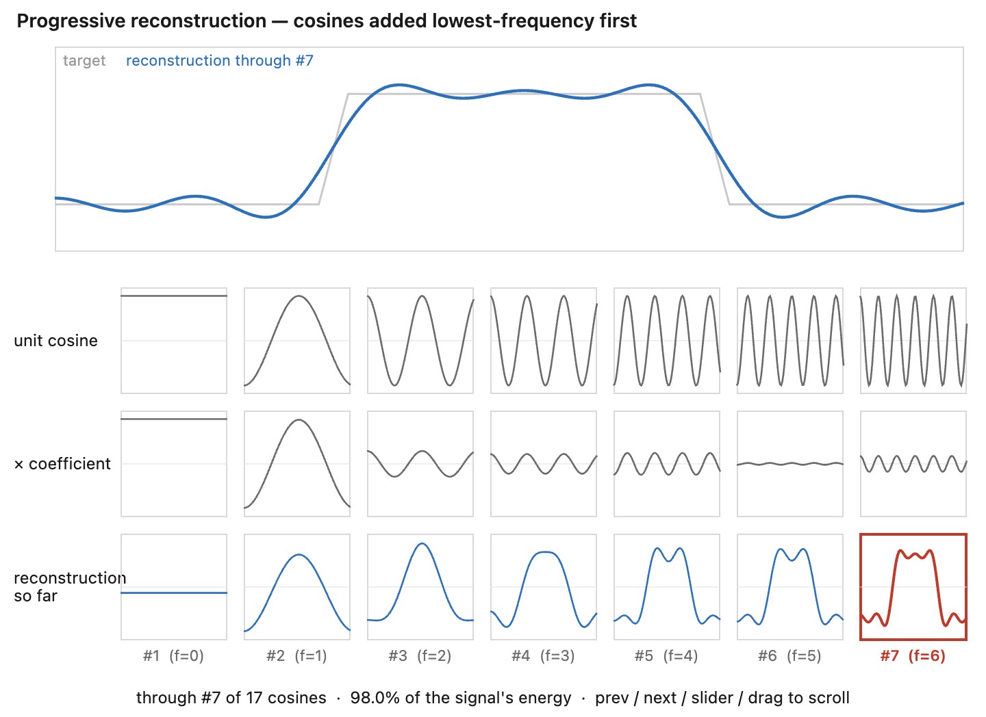
We can add waves in increasing frequency order, or in decreasing contribution to signal energy (Figure 6.3.12). A low-pass reconstruction of a sharp pulse rings near its edges. For a continuous discontinuity, Fourier-series overshoot persists while its affected region narrows, the Gibbs phenomenon. A finite DFT with every coefficient restored reproduces the original samples exactly; the intermediate ringing must disappear at those samples.
The same two orderings carry over to an image (Figure 6.3.13). Add the waves back lowest-frequency first and the picture blurs in from coarse to fine, the smooth tone first and the sharp detail last; sort them instead by amplitude, largest first, and it assembles from the highest-energy strokes down. Either way the striking part is how few waves it takes: a handful already give a recognizable image, because a natural photograph packs most of its energy into a small number of low frequencies. That concentration is exactly what image compression exploits, keeping the large coefficients and discarding the swarm of tiny ones, and it is the thread we pick up again with the DCT and JPEG.
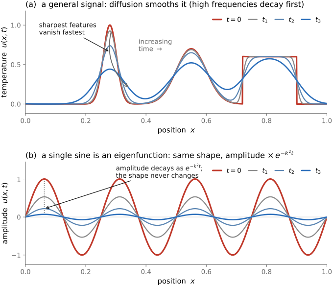
This Fourier transform was not invented for images. Jean-Baptiste Joseph Fourier (1768–1830) was trying to solve heat diffusion in a one-dimensional rod with a given initial temperature profile, and the governing equation was a coupled mess. His move, in 1807, was to write the temperature as a sum of cosines, and in that basis the heat equation diagonalizes: each frequency evolves entirely on its own, and a single cosine simply decays exponentially in time ($\propto e^{-k^2 t}$), the highest frequencies fastest, so any profile smooths out. The cosines are the eigenfunctions of the Laplacian (the diffusion operator), the same reason Fourier diagonalizes our convolutions. Notice what separation of variables has handed us: the two canonical solution families of linear differential equations meeting in one problem, sine waves in space and exponentials in time. The spatial sinusoids set the basis; their amplitudes decay as $e^{-k^2 t}$, the finest ripples dying first, so a general profile melts smooth while a single sine merely fades in place without changing shape (Figure 6.3.14). The lesson reaches far past heat: for almost any linear ordinary differential equation (ODE) or partial differential equation (PDE), find the eigenbasis and a coupled system decouples into independent scalar equations whose solutions are plain exponentials ($e^{\lambda t}$) or, for oscillatory systems, sine waves. Diagonalizing is the win.
Everything above assumed a grayscale image, one coefficient per wave. Color needs nothing new: run the same transform on each channel, giving three sets of coefficients. Every statement here holds channel by channel, so we develop it in grayscale and apply it thrice.
The matrix view makes the computation especially concrete. Put one sampled basis wave in each row of the transform matrix, using the complex conjugate for the forward projection. Multiplying that row by the image computes one coefficient. There is no separate linear system to solve because the basis waves are orthogonal; normalization supplies the inverse scale. The same basis works for every circular convolution, so changing the blur changes the diagonal gains rather than the basis itself.
6.3.5 Reading an image's Fourier transform⧉
For a 2-D image the recipe is the same with two frequency indices $(u, v)$, horizontal and vertical, so the transform is itself an image, the same size as the original, with a value at each frequency. We display it as two pictures: a magnitude (how much of each frequency is present) and a phase (where each wave sits). A handful of properties make these readable.
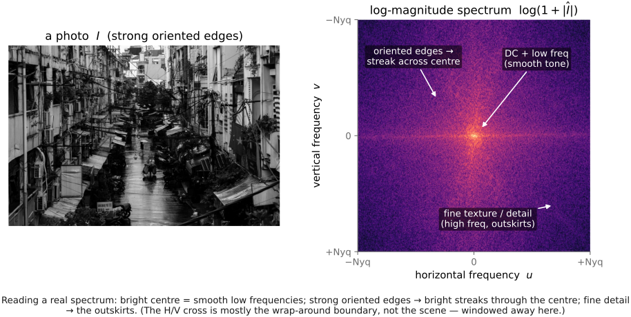
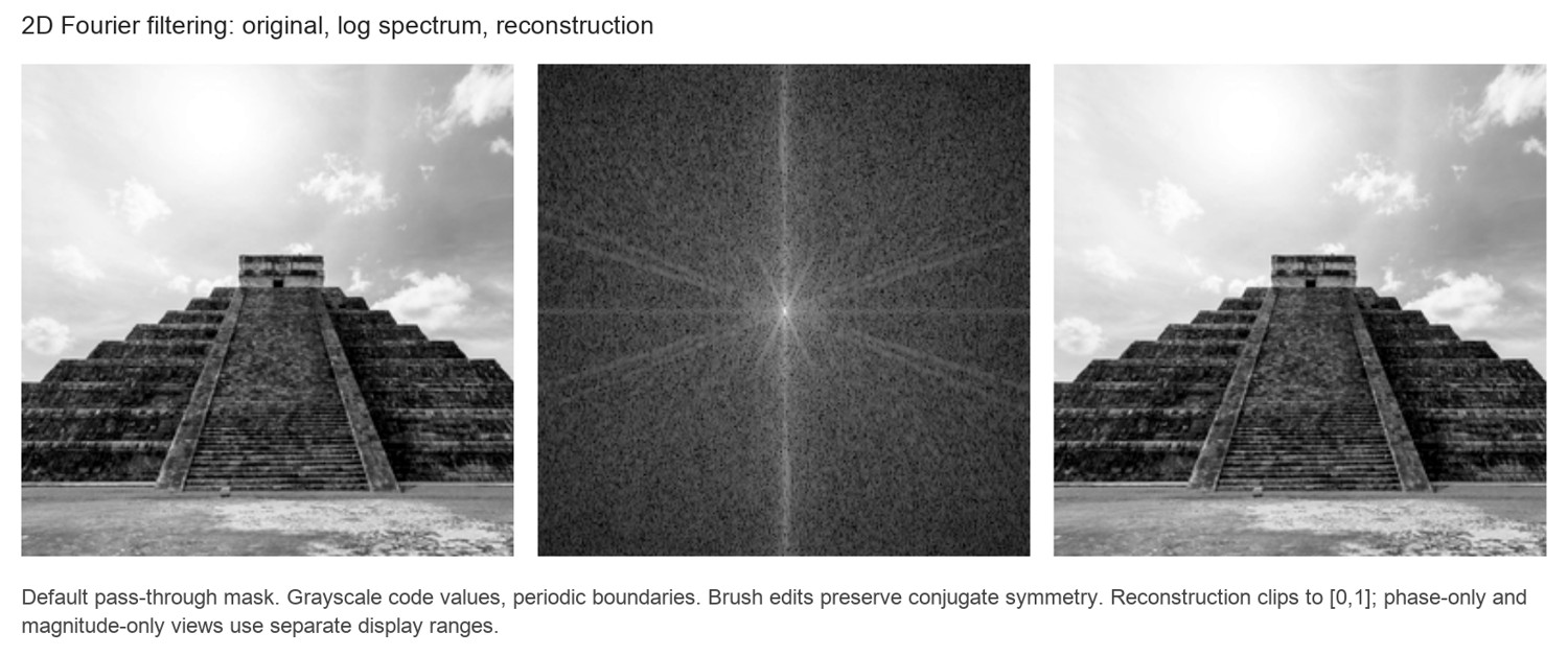
First, a real image has a conjugate-symmetric spectrum: the coefficient at frequency $(u, v)$ is the mirror of the one at $(-u, -v)$, so half the coefficients are redundant and the magnitude image is point-symmetric about its center. The very low frequencies (slow, large-scale variation) sit near the center; the high frequencies (fine detail, sharp edges) sit out toward the corners. Many photographs have larger individual coefficients at low frequencies, so a typical per-coefficient magnitude spectrum is bright in the middle and dim at the edges, often with bright streaks where strong oriented structure (a horizon, a picket fence) lives. Set a real photograph beside its log-magnitude spectrum and you can read these correspondences off directly (Figure 6.3.15): the bright center is the smooth tone, oriented scene edges show up as bright streaks through the center, and fine texture fills the outskirts. (Beware: the cyclic wrap-around assumption itself injects a cross of horizontal and vertical power, from the discontinuity where the image's left edge meets its right; serious analysis windows the image first to suppress it.)
A second reading aid is to manipulate the spectrum and watch what returns. Because filtering is multiplication in frequency, we can low-pass or high-pass a real photo by hand: transform it, multiply the spectrum by a mask, a disk that keeps only the center, or its complement that keeps only the outside, and transform back (Figure 6.3.17). Keep the center and the fine detail is gone: a smooth, blurred image, since the detail lived in the high frequencies we deleted. Keep the outside and only the edges and texture survive, the smooth tone subtracted away. This is the convolution theorem turned into an operation you can watch.
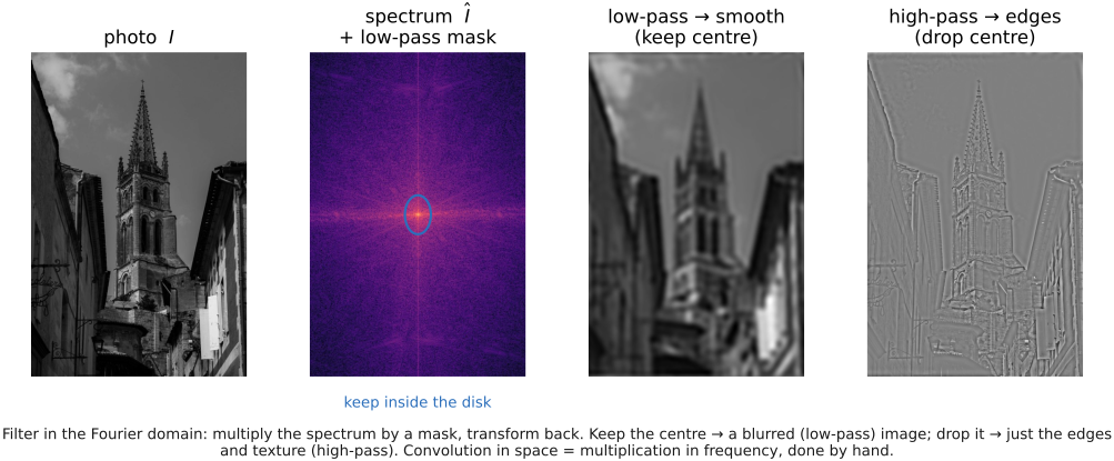
This low-pass/high-pass split is so useful that retouchers reinvented it by hand, without ever transforming to the frequency domain. The technique is called frequency separation, and it is a staple of portrait and product editing in Photoshop: blur a duplicate layer to isolate the low frequencies (the smooth tone and color transitions), subtract that from the original to recover the high frequencies (the pores, hairs, and fine texture) on a second layer, and then edit each independently: even out blotchy skin tone or color on the low-frequency layer while leaving pore detail perfectly crisp on the high-frequency layer, or vice versa. It is exactly the two-band decomposition above (a low-pass plus its high-pass complement, which sum back to the original), arrived at pragmatically by photographers who needed to touch tone and texture separately; the major retouching tutorials walk through the layer recipe in detail (Frequency separation (Photoshop retouching technique)).
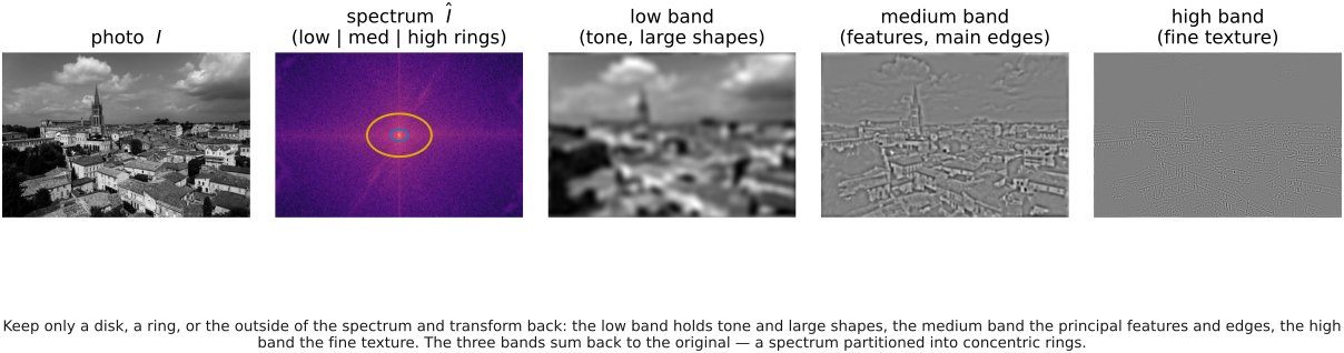
Splitting the Fourier coefficients into three disjoint regions gives low, medium, and high frequency components (Figure 6.3.19). Their sum reconstructs the image exactly because each coefficient belongs to one region. The visual importance and energy of a band depend on the image and cutoffs. Laplacian pyramids offer a related multiscale representation with overlapping responses rather than sharp frequency partitions (Chapter 6.6, Pyramids and wavelets).
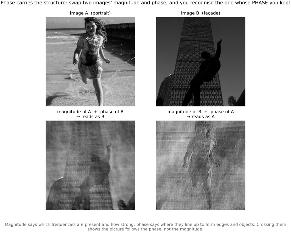
Phase describes how waves line up to form edges and objects. Swapping the phases of two photographs often makes each reconstruction resemble its phase donor (Figure 6.3.21). Magnitude still matters: it determines contrast and the strength of each frequency, and can contain substantial information about shape and texture. A coefficient of zero magnitude has no defined phase.
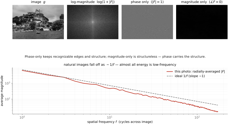
Try the swap on two photographs with broadly similar magnitude spectra. Their common spectral statistics make the importance of phase especially visible. It is a useful demonstration, not a guarantee for arbitrary images: replacing the magnitude by zeros, or retaining only a few frequencies, destroys the picture regardless of its phase.
Phase specifies the alignment of the waves; magnitude specifies their strength. Phase swaps between typical photographs often preserve recognizable structure from the phase donor, but accurate reconstruction requires both.
A circular shift of a finite image changes only phase: shifting by $(d_x,d_y)$ multiplies each coefficient by $e^{-2\pi i(ud_x/W+vd_y/H)}$, whose magnitude is one. A translation of an unbounded signal obeys the same rule. Translating and cropping a photograph also changes its contents, so its magnitude spectrum need not stay fixed. General convolutions can change magnitude as well as phase.
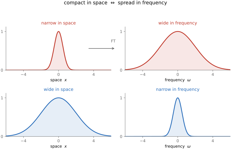
Fourth, the compact-in-space / spread-in-frequency tradeoff. A narrow, sharply localized blob in the image has a wide spectrum, and a wide smooth blob has a narrow one (Figure 6.3.22). A Gaussian makes this exact: the narrower the Gaussian in space, the wider its Fourier transform, which is itself a Gaussian. You cannot be compact in both domains at once. This locality-versus-frequency tradeoff is a genuine uncertainty principle, and it is the reason we will later want pyramids and wavelets, which sit halfway between the pixel and Fourier representations to buy some localization in both.
View each inverse-transformed band on its own before adding them. The low band gives a blurred arrangement of large light and dark regions. The high band often looks like faint signed texture on a gray background because a display offset is needed to see negative values. A faint-looking band can still matter at an edge, so compare both its energy and the visual effect of omitting it. Returning the three disjoint coefficient sets to the spectrum reconstructs the original; clipping the displayed band images before summing would not. This separates the decomposition from its visualization (Figure 6.3.19).
6.3.6 A small bestiary of transforms⧉
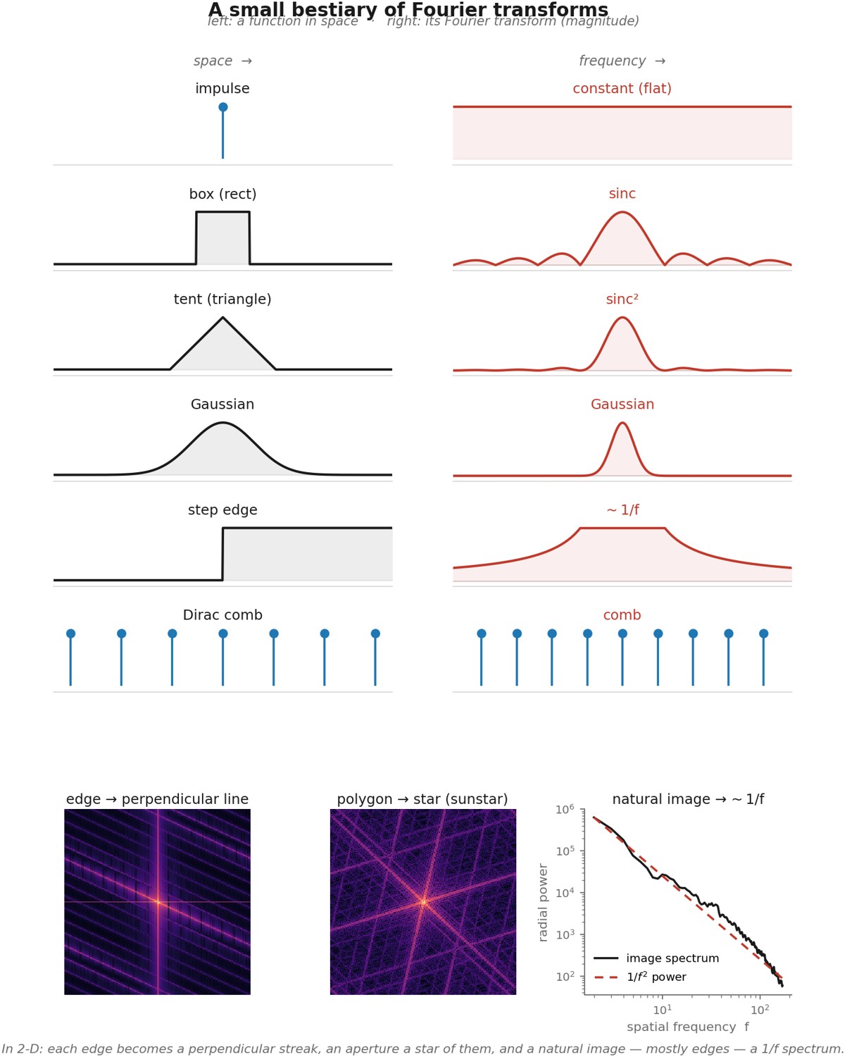
A handful of shapes recur so often that knowing their transforms by sight is most of the working intuition. Each pairing reinforces the space–frequency tradeoff (narrow here = wide there) and connects back to operations we already use (Figure 6.3.23).
- Impulse (delta) ↔ constant. A single bright point contains every frequency in equal measure, a flat spectrum; conversely a constant (DC) is a single spike at zero frequency. This is why a point source probes a system's whole frequency response: the PSF's transform is the optical transfer function (OTF); its normalized magnitude is the MTF.
- Box (rect) ↔ sinc. A unit-area continuous box of width $w$ transforms to $\operatorname{sinc}(w f)$, a central lobe with side-lobes that decay only as $1/f$. Wider box → narrower sinc. A hard frequency cutoff therefore produces a ringing spatial kernel. A spatial box average has nonnegative weights and cannot overshoot a step.
- Tent (triangle) ↔ sinc². A triangle is a box convolved with itself, so its transform is the box's squared, $\operatorname{sinc}^2$, whose side-lobes now fall as $1/f^2$, giving stronger high-frequency attenuation. Both spatial box and tent averages have nonnegative weights and cannot overshoot a step.
- Gaussian ↔ Gaussian. The Gaussian is (up to scale) its own transform: a smooth positive shape in both domains, and a narrow Gaussian ↔ a wide one, the space–frequency tradeoff in its purest form.
- Step edge ↔ ~$1/f$. A sharp step's spectrum falls off as $1/f$ (its derivative is an impulse, flat in frequency; integrating divides by $f$). The full transform also includes a DC term; the $1/f$ statement describes its nonzero-frequency component.
- Comb ↔ comb. A train of impulses transforms to another train of impulses, the fact behind sampling, in the next chapter.
An infinite straight edge varies only perpendicular to itself, so its transform is supported on the corresponding frequency line. Finite edges broaden this support. Aperture edges similarly help explain the directions of diffraction spikes, but the observed intensity is the squared magnitude of the transform of the entire aperture. Many natural photographs have an approximately $1/f$ average amplitude spectrum, or $1/f^2$ power spectrum, over a limited range. This is an empirical statistical regularity. In two dimensions, larger annuli contain more coefficients: a $1/f^2$ power spectrum gives roughly equal non-DC energy per octave, not almost all energy in the lowest octave.
Natural photographs often have approximately $1/f$ average Fourier amplitude over a range of scales. Distinguish amplitude from power, and average power per coefficient from total energy in a frequency band. The image mean can dominate total energy without explaining its visible detail.
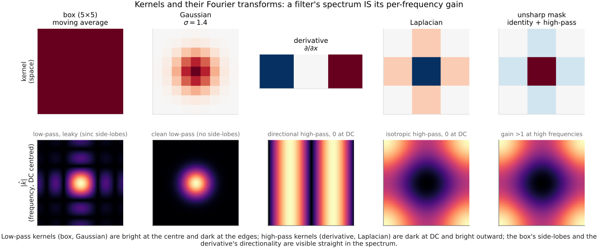
The frequency response also distinguishes practical kernels (Figure 6.3.24). A sampled box has zeros and side lobes, so it suppresses some high frequencies much less than others. A continuous Gaussian has a Gaussian transform; sampling and truncating it perturb that ideal. Derivatives kill DC, but their discrete responses depend on the stencil: a centered difference also vanishes at Nyquist. A Laplacian suppresses constant regions, while unsharp masking raises the gain of selected detail frequencies above one. Use the transform of the actual discrete kernel when predicting an implementation.
6.3.7 Optics and Fourier⧉
Optics performs a Fourier transform physically. Light is a wave, wave optics is a story about sines and cosines, and two everyday phenomena are Fourier transforms outright.
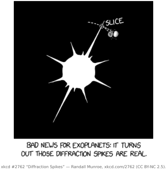
The first is diffraction. Send light through a small aperture and look far away, or in a lens's focal plane: you see the Fourier transform of the aperture (its squared magnitude). A round opening gives the Airy disc and rings; a polygonal iris gives a sunstar whose every spike is the transform of one straight blade-edge, a line of ripples perpendicular to it, so the star reads out the shape of the diaphragm (Figure 6.3.2). The optics does it for free, the same physics by which a smaller aperture diffracts, and blurs, more.
Under coherent illumination, a transparency at the front focal plane of a lens produces its field-amplitude Fourier transform at the back focal plane, up to coordinate scaling and phase factors. A mask in this Fourier plane multiplies that amplitude spectrum. A second lens transforms it again, giving the filtered field with spatial inversion in a 4f system. The detector then measures squared magnitude. This is amplitude filtering; it is not the intensity convolution model of an ordinary incoherently illuminated photograph.
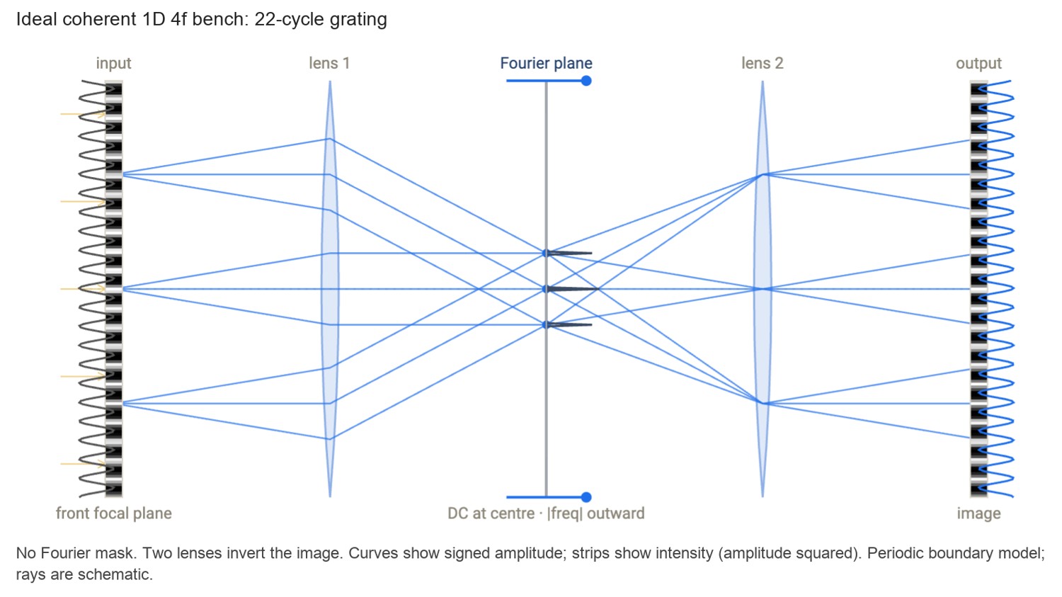
In the Fourier plane, the center represents the zero-frequency field component and positions farther away represent finer spatial variation. Blocking the center suppresses low-frequency amplitude; blocking the outside suppresses fine-scale amplitude; a directional opening selects orientations. This gives a physical interpretation of the masks used in the numerical demonstration. The field must still be propagated and squared to predict a detector image.
6.3.8 MTF: a lens's frequency response⧉
For an incoherent, locally shift-invariant imaging system, let $g$ be the intensity PSF. Its Fourier transform is the optical transfer function (OTF), which may be complex. The modulation transfer function is its normalized magnitude:
It measures contrast transfer but omits phase shifts. An ideal finite-aperture lens is still diffraction-limited: its MTF falls with frequency and reaches a cutoff. Only an ideal impulse PSF would retain unit contrast at every frequency. Lens MTF can vary across the field and with orientation. See Chapter 22.1, Aberrations and optical challenges.
6.3.9 The fine print: two limitations of Fourier⧉
Two implementation choices deserve attention: boundary handling and spatial locality.
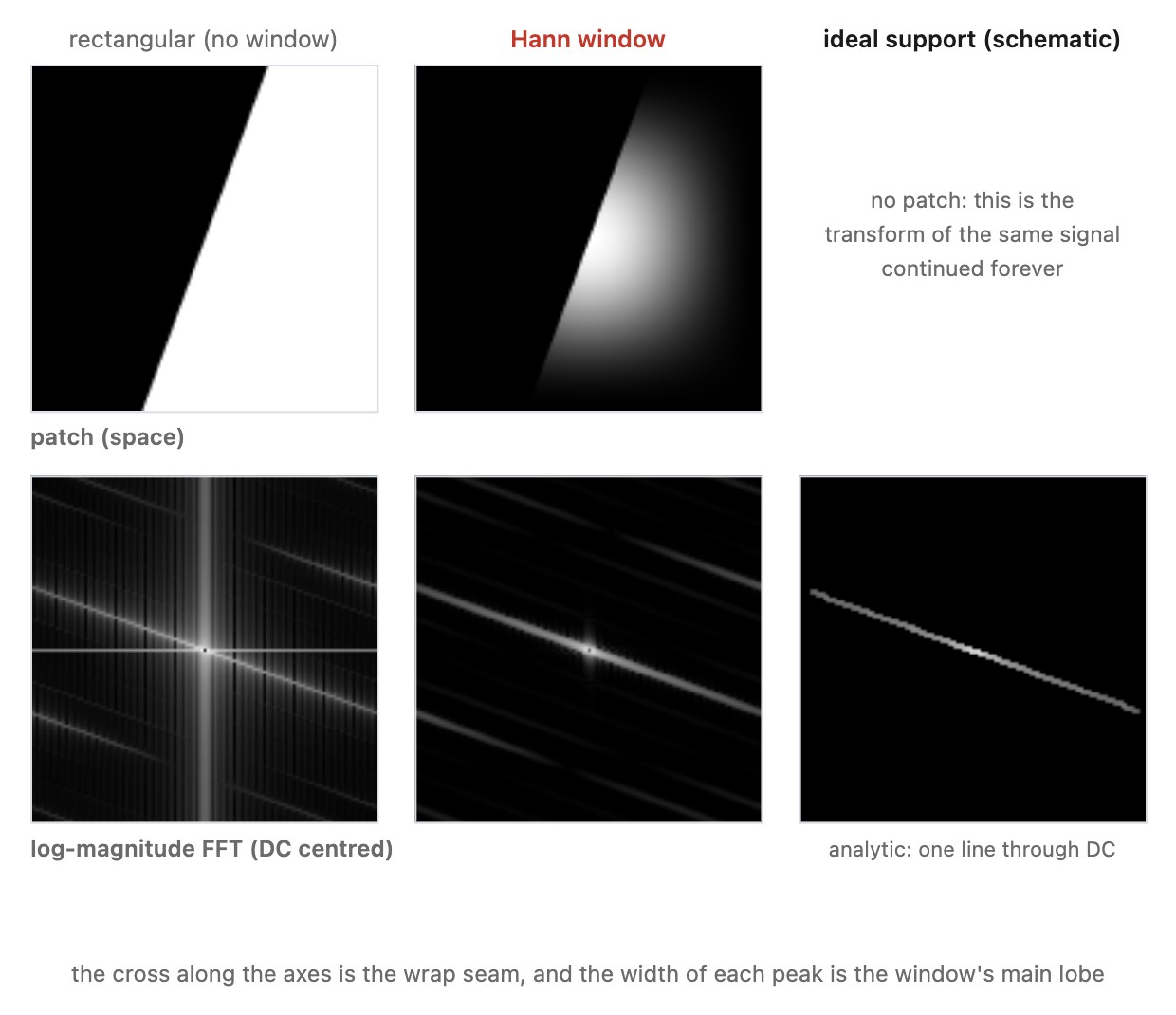
The finite DFT uses a periodic basis. Multiplying spectra and transforming back computes circular convolution. To compute linear convolution of finite arrays, zero-pad enough that the circular copies cannot overlap, then crop the desired result. Reflection or replication is another extension model and must be implemented explicitly. For spectral measurement, a mismatch at the period boundary causes leakage; tapering the patch reduces that mismatch but changes the measured signal.
Each finite DFT basis wave spans the whole image. One coefficient describes a global frequency component, so it cannot directly locate a texture in a particular corner. The complete complex spectrum still preserves every pixel and its location. Pyramids and wavelets make spatially localized frequency information easier to manipulate (Chapter 6.6, Pyramids and wavelets).
The DFT diagonalizes circular convolution exactly. With sufficient zero padding it also computes finite linear convolution exactly. Each basis wave is global, while the complete spectrum retains all spatial information. Choose the boundary extension to match the image operation.
A small bright spot illustrates the localization issue. Its contribution is spread across many Fourier coefficients. Moving that spot changes the phases of those contributions even when their magnitudes stay the same. The full complex transform therefore retains position information and can reconstruct the image; the difficulty is that a coefficient describes a wave over the whole image rather than a feature at one location. A windowed transform or wavelet coefficient restricts the spatial region at the cost of less precise frequency localization. That is the reason to introduce a localized representation, not a claim that Fourier transformation loses the positions of objects.
6.3.10 Windowing: the price of measuring a real spectrum⧉
The first of those caveats, the cyclic-boundary leakage, is mostly a curiosity when we use Fourier to think, but it becomes a genuine hazard the moment we measure. So we pause on the one fix, and on what that fix costs.
When opposite edges of a patch disagree, its periodic extension has a seam. The seam spreads spectral energy, often producing an axis-aligned cross. Multiplying by a Hann or Blackman taper reduces the seam by approaching zero at the boundaries. A Hamming window reduces leakage too, but its endpoints are nonzero. These are choices of spectral measurement window, not replacements for padding in convolution.
The window is not free, and the tradeoff is the whole story. A taper suppresses the side-lobe leakage, but in exchange it broadens every spectral peak: each sharp spike in the true spectrum is convolved with the window's own transform, so its main lobe widens. And because the taper discards the data near the borders (that is the entire point), it throws away signal and shrinks the effective patch. The two effects trade off directly: a narrower, more aggressive window kills more leakage but blurs frequency resolution and wastes more of the patch, while a gentler window keeps resolution and data but lets more of the cross survive. The named windows are just different points on that curve: Hann, Hamming, and Blackman differ precisely in how they balance main-lobe width against side-lobe height, Blackman buying the lowest side-lobes at the cost of the widest main lobe.
For quantitative measurements, record the window and its normalization. Amplitude estimates depend on the mean window weight; noise-power estimates depend on mean squared weight. Windowing broadens peaks and reduces boundary contributions, so it can hide real features near a border. A periodic test pattern sampled over complete periods may need no taper. An MTF or noise-power procedure should specify its own measurement protocol.
6.3.11 Application preview: can we deblur, given the blur?⧉
We can finally settle the promise. Suppose we know the blur, the kernel $g$ the optics applied, and we are handed the blurred image; this is non-blind deconvolution (the harder blind case, where the kernel is unknown, waits for a later chapter). The Fourier view makes the question crisp. In the frequency domain, blurring multiplied each frequency of the sharp image by the kernel's eigenvalue: $\hat I_\text{blur} = \hat I_\text{sharp} \cdot \hat g$. To invert, just divide it back out:
This is inverse filtering. It is exact for noiseless data wherever the response is nonzero. A blur diagonalized into per-frequency multiplications is undone by per-frequency divisions. So why is deblurring not a solved problem?
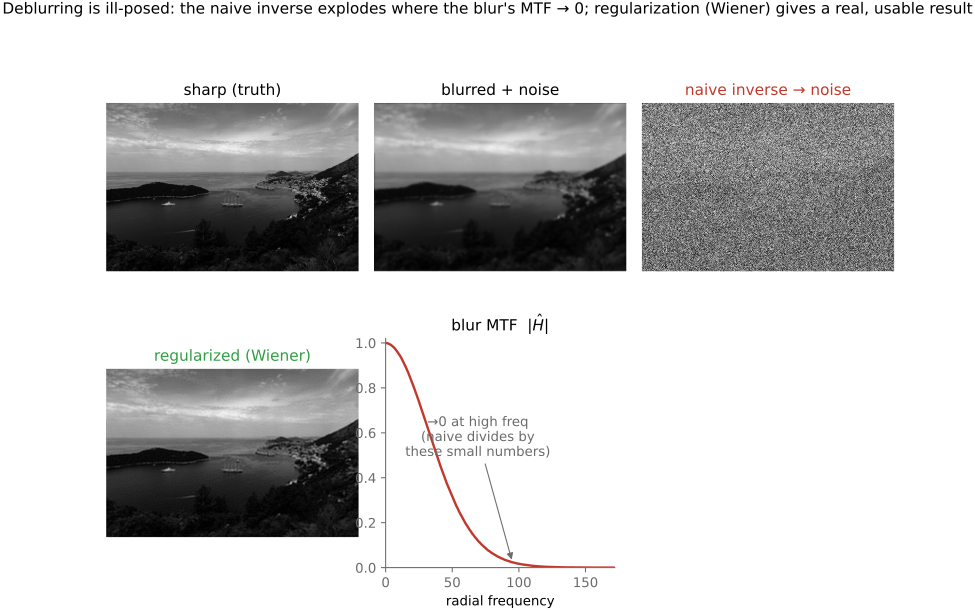
Because of the one number we said decides everything: how close the eigenvalue is to zero. A blur is a low-pass filter, so $\hat g$ is large at low frequencies but tiny, near zero, at exactly the high frequencies the blur destroyed. Dividing by a near-zero number is catastrophic. And real images carry noise: a little random grain the sensor added after the blur, so that what we actually observe is $\hat I_\text{blur} = \hat I_\text{sharp}\cdot\hat g + \hat n$. Divide that through and we get $\hat I_\text{sharp} + \hat n / \hat g$: the genuine signal comes back, but the noise term is divided by $\hat g$ as well. At a high frequency where $\hat g \approx 0.01$ the blur attenuated the signal a hundredfold, yet it never touched the noise, which was added afterward, so dividing by $0.01$ now amplifies that noise a hundredfold. The inverse filter faithfully reconstructs the signal and, in the same stroke, explodes the noise; the result is a sharp-looking image drowned in colorful high-frequency garbage (Figure 6.3.28). This is the central difficulty of deblurring, and the Fourier picture diagnoses it exactly: inverse filtering is unstable precisely where the blur was strong.
A Wiener filter balances inversion against noise amplification. For independent, zero-mean stationary signal and additive noise with power spectra $S_I$ and $S_n$, the minimum-mean-square-error linear estimate uses
The star denotes complex conjugation. Where the signal dominates, the factor approaches $1/\hat g$; where noise dominates, it suppresses the measurement. Frequencies with no measured information cannot be recovered by division. This formula depends on the assumed spectra and boundary model; it does not claim to be the best nonlinear estimator. Chapter 7.1, Imaging as Bayesian inference with probabilistic priors develops the statistical interpretation.
In the Fourier basis a convolution is diagonal: it multiplies each frequency by one number (the kernel's complex response, the OTF), so undoing it is a per-frequency division. The whole stability question becomes local to each frequency: how near zero is that number? Blur is low-pass, so its response is tiny at exactly the high frequencies it destroyed; the lower a frequency's coefficient, the more its noise is amplified on inversion. That is why naive deblurring fails worst precisely where the blur was strongest, and why a Wiener / regularized filter stops dividing once the signal drops below the noise floor.
6.3.12 Convolution by FFT⧉
The fast Fourier transform (FFT) computes an $N$-sample DFT in $O(N\log N)$ operations. It changes the cost of the transform, not its definition. This makes spectral multiplication a useful way to compute large convolutions.
Direct convolution costs $O(NK)$ for $N$ output pixels and a kernel with $K$ taps. FFT convolution costs $O(P\log P)$ for a padded array with $P$ elements. The required padding grows with the kernel, so the cost is not completely independent of kernel size. Small kernels usually favor direct convolution; separable kernels have a cheaper direct implementation.
For zero-extended input of size $H\times W$ and a kernel of size $K_h\times K_w$, use transform dimensions at least $H+K_h-1$ and $W+K_w-1$. Here is full convolution with both arrays stored from index zero:
P = efficient_fft_size(H + Kh - 1, W + Kw - 1)
A = zeros(P); A[0:H, 0:W] = image
B = zeros(P); B[0:Kh, 0:Kw] = kernel
full = real(ifft2(fft2(A) * fft2(B)))
full = full[0:H+Kh-1, 0:W+Kw-1]
# For a centered odd kernel, crop from (Kh//2, Kw//2)
same = full[Kh//2:Kh//2+H, Kw//2:Kw//2+W]
The inverse includes its usual normalization. No fftshift is needed in this convention. For reflected boundaries, extend the image first and adjust the crop. Check an impulse and an asymmetric kernel to catch shifts and accidental correlation.
Running sums compute box filters in linear time. Repeated boxes and recursive filters approximate a Gaussian efficiently, while a separable finite Gaussian can be computed exactly in two passes. Compare approximation error as well as runtime. An arbitrary large PSF is a stronger case for FFT convolution (Chapter 29.1, Algorithmic speedups).
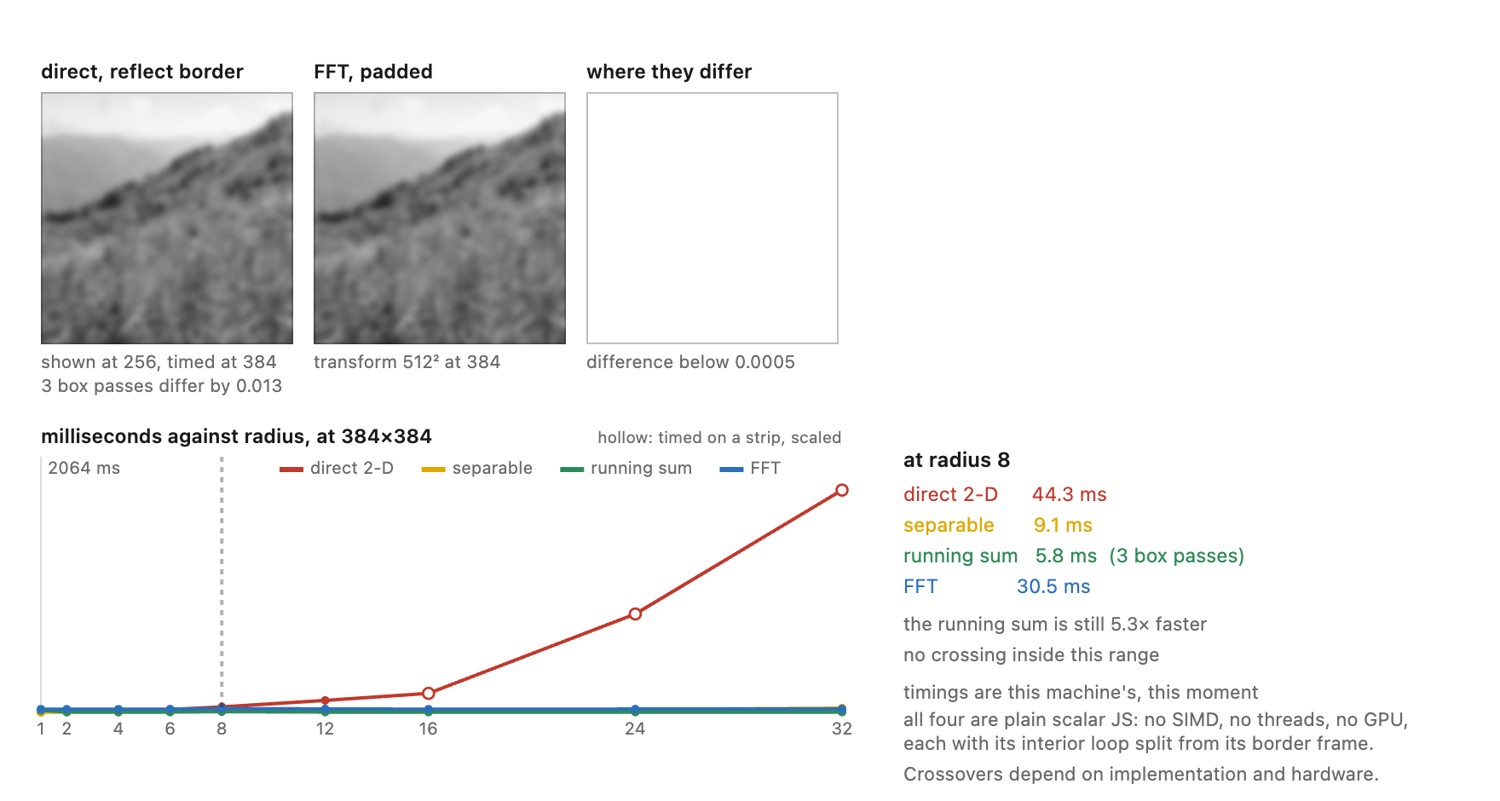
The FFT method pays for transforming a padded image, transforming a padded kernel, multiplying their coefficients, and transforming the result back. A small direct kernel performs only a few multiplies per pixel and avoids those transforms, so asymptotic complexity alone does not choose the faster method. A large nonseparable point-spread function can reverse that comparison. If many images use the same kernel, its transform can be reused. If the kernel is separable, compare against two one-dimensional direct passes rather than the more expensive two-dimensional baseline. Padding, boundary handling, and reusable transforms belong in the performance comparison as well as in the correctness check.
The radix-two Cooley–Tukey construction splits an even-length transform into transforms of the even-indexed and odd-indexed samples. Each half is reused when forming two groups of outputs, with known complex phase factors accounting for the odd positions. Recursing on the halves gives a logarithmic number of stages with linear work per stage. This is why the FFT computes the same coefficients as the direct sum with far fewer operations; it is not an approximate transform. Other factorizations handle other lengths.
Recap: big lessons of this chapter
Express a linear operator in a basis where it becomes diagonal. A coupled, hard-to-invert operation in one representation can be a list of independent scalar multiplications in another, and scalars are trivial to understand, compose, and invert. Fourier diagonalizes convolution, turning a blur into per-frequency multiplication. This is not a one-off trick: it is the single most reusable move in applied linear algebra, and it returns for differential equations (the heat equation, below), for principal components, and for nearly every inverse problem in this book. The idea is already visible in the smallest possible case, a $2\times2$ matrix (Figure 6.3.3).
Phase specifies the alignment of the waves; magnitude specifies their strength. Phase swaps between typical photographs often preserve recognizable structure from the phase donor, but accurate reconstruction requires both.
Natural photographs often have approximately $1/f$ average Fourier amplitude over a range of scales. Distinguish amplitude from power, and average power per coefficient from total energy in a frequency band. The image mean can dominate total energy without explaining its visible detail.
The DFT diagonalizes circular convolution exactly. With sufficient zero padding it also computes finite linear convolution exactly. Each basis wave is global, while the complete spectrum retains all spatial information. Choose the boundary extension to match the image operation.
In the Fourier basis a convolution is diagonal: it multiplies each frequency by one number (the kernel's complex response, the OTF), so undoing it is a per-frequency division. The whole stability question becomes local to each frequency: how near zero is that number? Blur is low-pass, so its response is tiny at exactly the high frequencies it destroyed; the lower a frequency's coefficient, the more its noise is amplified on inversion. That is why naive deblurring fails worst precisely where the blur was strongest, and why a Wiener / regularized filter stops dividing once the signal drops below the noise floor.