22.7 Special optics⧉
Every lens in the last two chapters was trying to do the same thing: image a flat scene onto a flat sensor, with straight lines staying straight, every color in focus together, sharply, across the whole frame. Each design in this chapter deliberately gives up one of those defaults in order to gain a specific capability. Tilt the lens and the plane of sharp focus is no longer parallel to the sensor, which lets you lay focus along a tabletop or slice a thin diagonal wedge. Stop insisting on rectilinear projection and you can swallow a 180-degree field in one frame. Replace refraction with reflection and a long telephoto folds into a stubby tube whose reflecting surfaces add no refractive chromatic aberration. Squeeze the image with cylinders and a wide picture fits a narrow frame. Each is a trade, made knowingly, and several of the trades have a computational counterpart: software can finish what the optics deliberately left undone (un-warp a fisheye), or imitate in pixels a look the glass produced for free (anamorphic flares, smooth bokeh). The chapter closes by pushing that trade to its limit: discard most of the glass and keep only its effect on the wavefront, which is the road from the Fresnel lens to the metalens, and the on-ramp to flat optics in the Advanced part.
22.7.1 Tilt-shift and the Scheimpflug principle⧉
A normal lens is mounted with its optical axis perpendicular to the sensor and centered on it. A tilt-shift lens (also called a perspective-control lens) breaks that rigid mounting in two independent ways, and the two do entirely different jobs.
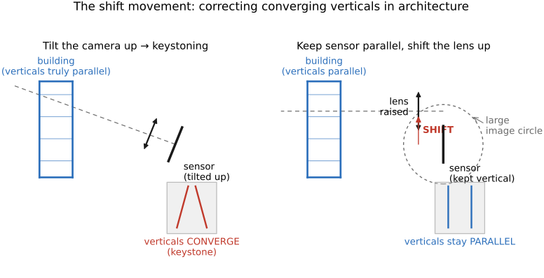
Shift slides the lens parallel to the sensor, keeping the axis perpendicular. Because the lens projects a circular image and the sensor samples a rectangle out of it, shifting moves the rectangle to a different part of the image circle, as if you had cropped off-center from a wider view. The payoff is perspective control: point a camera up at a building and the verticals converge (the classic keystoning); raise the lens by shifting instead, keep the sensor vertical, and the building's edges stay parallel, because the projection plane never tilted. For a panorama, moving the sensor behind a stationary lens preserves the viewpoint. Shifting the lens on a fixed camera body moves the entrance pupil and can introduce parallax, especially for nearby objects. A lens-mounted support with rear shift or a compensating camera movement addresses this distinction. The only cost is that the lens must throw a much larger image circle than the sensor needs, so there is room to shift into.
Tilt is the more surprising motion: rotate the lens so its axis is no longer perpendicular to the sensor. For an ordinary lens, the plane of sharp focus is parallel to the sensor, a flat slab at one distance. Tilt the lens and that plane also tilts, but not by the same angle, and it pivots about a line you can locate exactly. The Scheimpflug condition Scheimpflug 1904 says it cleanly: the lens plane, the sensor (image) plane, and the plane of sharp focus all intersect along a single line in space, the Scheimpflug line. When the lens is untilted, the three planes are mutually parallel and that line sits at infinity (the familiar slab-at-one-distance case); tilt the lens and the line swings in to a finite place, swinging the focus plane with it.
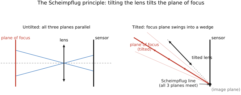
There is a companion rule for where the focus plane pivots, called the hinge rule. The plane of sharp focus rotates about a second line, the "hinge", at the intersection of the front focal plane and a plane through the lens center parallel to the sensor. In the thin-lens construction its distance from the lens center is $f/\sin\theta$, where $\theta$ is the lens tilt relative to the sensor. The practical reading is that the Scheimpflug line fixes the intersection of the focus plane with the lens, while the hinge line is the axis the focus plane swings around as you refocus: change focus and the focus plane rotates about the hinge like a trapdoor, rather than sliding back and forth as in a normal lens. Photographers use this two ways. Tilt to align the focus plane with a receding surface (a tabletop, a landscape foreground-to-background) and the whole surface is sharp at full aperture. Or tilt the other way, so the focus plane slices across the scene as a thin diagonal wedge, throwing most of the frame out of focus; that is the toy-town "miniature faking" look (the same look software now fakes with a graded blur).
Be precise about what tilt does and does not buy, because it ties straight into depth of field. Tilt redistributes the region of acceptable sharpness. It does not simply add a uniform thickness to the untilted depth of field: the in-focus region, normally a slab parallel to the sensor, becomes a wedge that fans out from the hinge line, thin near the camera and opening up far away. You are not getting more sharpness; you are choosing where to spend it (cross-reference Chapter 23.1, Bokeh, focus stacking, and depth-of-field control).
22.7.2 Fisheye and non-rectilinear projection⧉
A conventional lens is built to obey rectilinear projection: a straight line in the world images to a straight line on the sensor. The mapping from a ray's field angle $\theta$ (measured from the optical axis) to its radial distance $r$ from the image center is
This is exactly the pinhole/perspective projection from Chapter 2.2, Pinhole Image Formation and linear perspective, and it has a hard wall built into it: as $\theta$ approaches 90 degrees, $\tan\theta$ runs to infinity. A point at the edge of a 180-degree field would land infinitely far out. There is no hard 100-degree limit: rectilinear lenses and renders can cover wider fields, at the cost of increasingly stretched edge content and difficult optical design. The mathematical singularity occurs at a total field of 180 degrees along a dimension.
A fisheye lens abandons rectilinear projection and adopts a mapping that compresses the angle gracefully, trading straight lines for an enormous field, often 180 degrees or more. Two standard mappings appear:
The equidistant law $r=f\theta$ makes image radius simply proportional to field angle, so equal angular steps land at equal spacing, handy when you want to measure angles off the picture (scientific and surveillance fisheyes favor it). The equisolid-angle law $r=2f\sin(\theta/2)$ instead keeps equal solid angles of the scene mapping to equal areas on the sensor, which is what you want for whole-sky photography and is the common photographic fisheye. Both stay finite all the way to $\theta=90$ degrees and beyond. Neither $f\theta$ nor $2f\sin(\theta/2)$ runs off to infinity the way $f\tan\theta$ does, which is precisely why they can swallow a hemisphere.
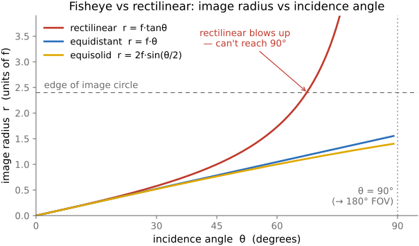
The geometry is clearest in a ray trace (Figure 22.7.4): send chief rays in from a wide cone of field angles and watch each bend through the front group to a finite spot on the sensor, equal angle steps landing at equal radial steps, while the rectilinear targets $f\tan\theta$ shoot off the sensor as the angle opens toward 90°.
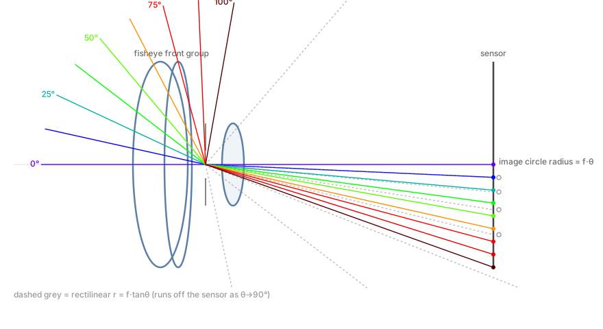
The strong barrel distortion of a fisheye, with straight lines bowing outward toward the frame edge, is not an aberration. It is the intended projection, the deliberate price of the wide field, and it is perfectly well-defined and invertible. Knowing the mapping law and $f$, software can re-project a fisheye frame back to rectilinear (or to any other projection: cylindrical, stereographic "little planet"), at the unavoidable cost of stretching the corners and discarding the field beyond what rectilinear can hold. This is the cleanest case in the whole part of optics and computation splitting the work: the glass gathers the impossible field, and the algorithm reshapes it afterward.
22.7.3 Mirrors: catadioptric and reflecting systems⧉
So far every element has refracted light through glass. Mirrors offer a different way to bend rays, with two structural advantages. First, a folded mirror path can pack a very long focal length into a short physical tube because light bounces back and forth instead of traveling straight through. Second, and more fundamentally, reflection has no dispersion: the law of reflection makes no reference to wavelength, so a mirror bends every color by exactly the same angle. A mirror system is therefore achromatic by construction. It has zero chromatic aberration, for free, where a refracting lens has to fight color with achromat doublets and exotic glass (cross-reference Chapter 22.2, Aberrations correction).
A catadioptric system (the name fuses cata-, reflective, with dioptric, refractive) uses mirrors and lenses together: mirrors do the heavy folding and the color-free focusing, while a few weak glass elements clean up the aberrations the mirrors leave behind. The compact mirror telephoto ("mirror lens", or reflex lens) is the photographic example, a 500mm or 1000mm lens shrunk to a short, wide barrel. It pays for that compactness with one unmistakable signature. Because a secondary mirror sits on the axis facing the primary, the lens has a central obstruction, and its effective pupil is therefore a ring, not a filled disk. Out-of-focus highlights are images of that pupil (from Chapter 23.1, Bokeh, focus stacking, and depth-of-field control), so on a mirror lens they render as bright doughnuts, hollow rings with a dark center, the instantly recognizable mirror-lens bokeh.
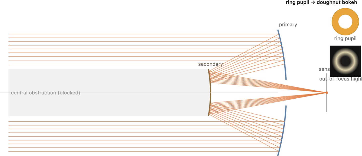
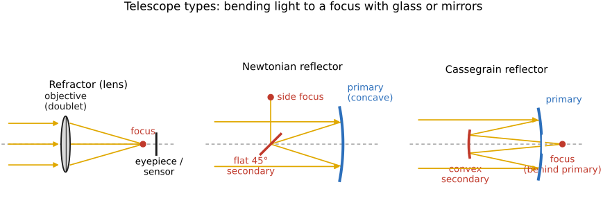
The same ideas scale up to telescopes. Pure reflectors, the Newtonian (a paraboloidal primary with a flat diagonal secondary) and the Cassegrain (a concave primary and a convex secondary folding the path back through a hole in the primary), use mirrors alone for large apertures where a glass lens of the same size would be unliftable and hopelessly chromatic. Catadioptric telescopes like the Schmidt-Cassegrain and the Maksutov add a refracting corrector at the front, a thin aspheric plate in the Schmidt design or a thicker meniscus in the Maksutov design, to fix the spherical aberration of an easy-to-make spherical mirror, marrying compactness to wide, sharp fields. At these apertures stray light becomes a first-order enemy, which is why large and space telescopes drive the glare and baffling discussion (cross-reference Chapter 22.10, Glare suppression).
22.7.4 Periscope / folded-lens design (smartphone telephoto)⧉
Every design in this chapter so far has faced an ordinary problem and solved it cleverly, but none faces a tighter packaging constraint than this: the phone body is only a few millimeters thick. A lens whose axis runs perpendicular to the screen can be no longer than that, which caps the optical focal length and with it the telephoto reach. The classic telephoto trick from Chapter 22.5, A short bestiary of classic designs helps: a positive group followed by a negative group pushes the rear principal plane forward, so the physical length is shorter than the focal length. But even with that, a long telephoto in a millimeter-thin package is a physical impossibility if you insist on a straight optical axis.
The periscope (or folded-optics) design breaks the insistence. A prism or mirror, placed right behind a small entrance window, bends the optical axis by roughly 90 degrees, turning it from perpendicular to the screen into parallel with the phone's face. The lens groups now lie sideways, running along the phone's width or length, where there is room for a long optical train. For a single fold followed by a sideways optical train, the sensor plane is perpendicular to the phone's back; further folds can change this orientation. Nothing about the optics is exotic; it is a telephoto lens system (real lens groups and optical focal length, with moving-group zoom only in modules designed for it) simply reoriented so its length runs the one direction where the device has space to spare.
The result is substantial. A folded module can deliver ~5× to 10× optical zoom (roughly 100–250 mm equivalent) within a compact phone module, though pupil diameter, sensor size, and packaging can still require a camera bump. Continuous or stepped zoom comes from moving internal groups in the usual way. Optical image stabilization is often handled by tilting or shifting the prism itself rather than floating a glass group, a compact, power-efficient approach. Apple's tetraprism, introduced in the iPhone 15 Pro Max, uses four internal reflections to fold the optical path, extending the effective path length still further within the same device width and reaching an equivalent focal length near 120 mm.
The folded design was popularized by the Huawei P30 Pro in 2019, and quickly taken up by Samsung (Galaxy S20 Ultra and successors) and then Apple. Earlier phones already offered separate short-telephoto optical modules as well as digital cropping. Folding extended the focal lengths that fit inside a phone; a 5× label usually compares that module with the main camera, rather than promising a continuous 1×–5× optical zoom. It is the direct hardware answer to a problem that was otherwise pushing toward ever-heavier computational magnification.
The periscope differs from the telephoto layout it complements. The telephoto design in Chapter 22.5, A short bestiary of classic designs shortens the physical length of the lens relative to its focal length, the same axis, just a shorter tube. The periscope does something independent: it reorients that (already-telescoped) tube so its length runs parallel to the device face rather than through it. In a modern phone telephoto module, both strategies are typically at work together.
There are real trade-offs to admit. The small entrance window and the losses in the prism limit the maximum aperture: a periscope module typically gathers less light than the phone's main wide camera. Each module covers a fixed or narrow zoom range, so a phone with, say, 1×, 3×, and 10× coverage uses three separate modules rather than one continuous zoom. And prism alignment and manufacturing cost add constraints that a simpler straight lens avoids. These are the known costs; the design is used because it provides useful telephoto reach within the device's packaging constraints.
22.7.5 Anamorphic optics⧉
An anamorphic lens deliberately images the world with different magnifications horizontally and vertically. A system of cylindrical elements, lenses curved in one direction only, squeezes the image horizontally, classically by a factor of $2\times$, while leaving the vertical untouched. The motive is historical and geometric: cinema wanted a very wide aspect ratio, but the film frame (and later the sensor) was nearer to square. Squeezing a wide scene horizontally by $2\times$ packs it onto the narrower frame; a matching anamorphic de-squeeze on the projector (or in post) stretches it back, restoring the correct wide proportions. You record the world horizontally compressed and undo the compression at the end, making fuller use of the available frame area than simply cropping a wide strip would.
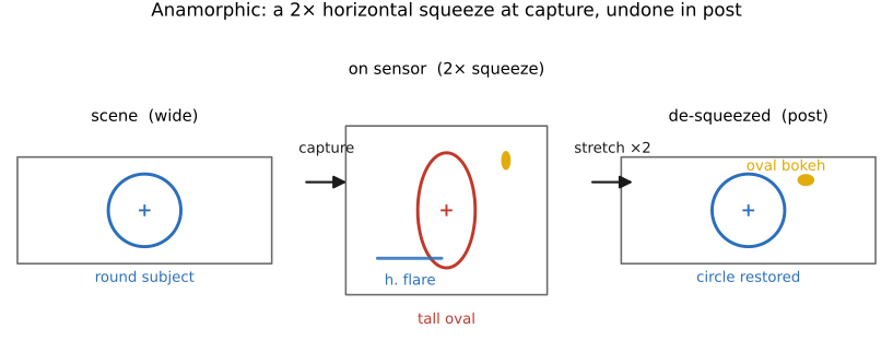
The cylindrical optics also produce side effects that later became part of the desired look. Because the aperture is effectively scaled differently in the two directions, out-of-focus highlights render as vertical ovals instead of round disks, the signature anamorphic oval bokeh. And bright sources throw long horizontal flare streaks (the famous blue lens-flare line across the frame). Neither is "correct" optics, yet both read as cinematic, and both are now imitated computationally (a depth-aware blur stretched into ovals, a synthetic horizontal streak) when a director wants the look without the lens.
22.7.6 Stereo (3D) lenses⧉
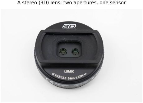
Another design repurposes the frame not to widen it but to split it. A stereo lens carries two small lenses side by side, a fixed baseline apart, each imaging onto one half of the same sensor, so a single exposure records a left/right stereo pair at once (Figure 22.7.8). It is a miniature two-camera rig packed into one mount: the two apertures see the scene from slightly different viewpoints, and that horizontal disparity is exactly the depth cue the two chapters on stereo and depth are built around (stereo). From the pair the camera can build a 3-D (MPO) image or a rough depth map with no moving parts and shared exposure timing, subject to the sensor's readout geometry; a rolling shutter can still assign different times to regions on different rows.
The price is steep in the usual ways. Each eye gets only half the sensor, halving resolution; the baseline is fixed and small, so the depth effect is weak beyond a few meters; and to keep both images sharp across the shared sensor the aperture is tiny and slow (the Panasonic Lumix G 3D lens is f/12), which starves it of light. These trade-offs are why single-lens stereo stayed a novelty while the industry moved to computational stereo, two ordinary cameras a wider baseline apart (phone multi-camera arrays), or a single camera with dual-pixel or learned monocular depth (depth-from-one-image), which supplies different depth cues: dual-pixel sensing measures pupil-split disparity, while learned monocular depth infers depth from image structure and priors without measuring a stereo disparity.
22.7.7 Macro, microscope objectives, and telescopes⧉
The lenses so far image distant scenes at small magnification. Push toward the opposite extreme, imaging something at life size or larger, and the design constraints reverse.
Macro photography means a magnification $m \ge 1$: the image on the sensor is at least as large as the object itself (1:1, or 2:1, or more). Recall the thin-lens conjugate relation $1/f = 1/u + 1/v$ from Chapter 2.2, Pinhole Image Formation and linear perspective. For a distant subject the image distance $v$ is essentially $f$; but at 1:1 magnification the object and image distances become equal and large ($u = v = 2f$), so the lens must rack far out from the sensor, and everything about the geometry runs the other way from normal shooting. Two consequences dominate. First, depth of field becomes razor-thin: at high magnification the in-focus slab can be a fraction of a millimeter, which is exactly why focus stacking (capturing many planes and merging the sharp pixels) lives in the depth-of-field chapter (cross-reference Chapter 23.1, Bokeh, focus stacking, and depth-of-field control). Second, flat-field correction matters more than usual: you are often photographing a flat subject (a stamp, a circuit board) and need it sharp corner to corner, so the residual field curvature an ordinary lens tolerates becomes intolerable, and macro lenses are designed flat.
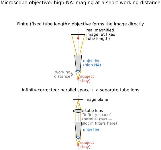
Microscope objectives and telescope objectives are not a different physics: they are the same compound-lens optimization from Chapter 22.4, Lens optimization, pushed to extreme corners of the design space. A microscope objective is a macro lens taken to very high magnification and very high numerical aperture, corrected for its own special demands: with achromat, fluorite, or apochromat correction grades, and plan objectives providing a flat field. Not every microscope objective has all these corrections. A telescope objective is the same machinery pushed toward very long focal length and very large aperture for faint, distant light. The lesson is continuity, not novelty: extreme magnification or extreme aperture is just the merit function weighted toward an extreme operating point, with the same aberrations to cancel and the same tradeoffs to pay.
22.7.8 Teleconverters⧉
A teleconverter (or extender) is the cheapest way to buy reach: a small secondary lens group that mounts between the master lens and the camera body and magnifies the image the master lens forms. A $1.4\times$ converter multiplies the focal length by $1.4$, a $2\times$ by $2$, turning a 300 mm lens into a 420 mm or a 600 mm without a new front element. It works by re-imaging the master lens's image at a larger scale, which is why its effects follow directly from that single fact: everything the master lens made is magnified, the good and the bad alike.
The first consequence is the f-number. A teleconverter magnifies the focal length but does not enlarge the physical aperture (the entrance pupil is set by the master lens), so the working f-number $N = f/D$ rises by the same factor: a $2\times$ converter costs two stops ($300$ mm $f/4$ becomes $600$ mm $f/8$), a $1.4\times$ costs one stop. That lost light is not a side effect but the same magnification seen in the aperture, and it is often the binding constraint: at $f/8$ many autofocus systems are at or past their low-light limit, which is why "does the body autofocus at $f/8$?" is the practical question a teleconverter raises. The second consequence is image quality. Because the converter magnifies the master lens's residual aberrations along with the image, it amplifies whatever softness, chromatic error, and field curvature the master lens had; a converter therefore performs well only on lenses that were designed with the headroom for it (the reason manufacturers certify particular teleconverter-and-lens pairings, usually top telephotos, and leave others uncoupled). The third is a happy one: a teleconverter does not change the master lens's minimum focus distance, so at closest focus it multiplies the magnification by its factor, turning a telephoto into a passable close-up lens.
Contrast a teleconverter with the free alternative, cropping. Both enlarge the subject; the difference is pixels. A $2\times$ converter spreads the subject across the full sensor, so if the master lens out-resolves the sensor you keep all your pixels on the subject; cropping the same framing from the bare lens throws three-quarters of them away. But if the lens is the limit rather than the sensor, the converter is magnifying blur and cropping would have given nearly the same result for free. A teleconverter can improve sampling of detail the master lens supplies, but its own aberrations, transmission, autofocus behavior, and the sensor's noise also enter the comparison. Judge matched final images rather than the nominal pixel count alone.
Most of this part is about removing defects. Two designs do the opposite. They add a controlled imperfection, because the imperfection is the desired image.
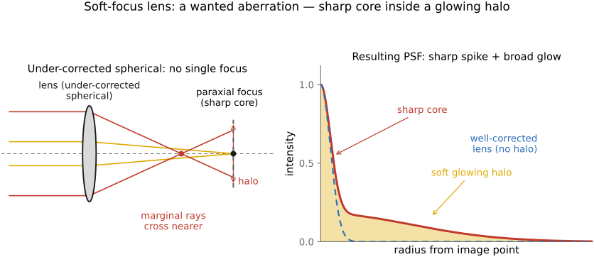
A soft-focus portrait lens deliberately leaves in under-corrected spherical aberration. Recall (forward-reference Chapter 22.2, Aberrations correction) that spherical aberration makes rays through the edge of the aperture focus at a slightly different distance than rays through the center. Left in on purpose, this overlays a sharp core with a soft glowing halo: every bright point picks up a luminous bloom, skin glows, highlights spread gently. It is a wanted aberration, dialed in (often adjustable, and often reduced by stopping down), giving a dreamy rendering no perfectly corrected lens can produce. The aberration the rest of the part fights to kill is here the entire selling point.
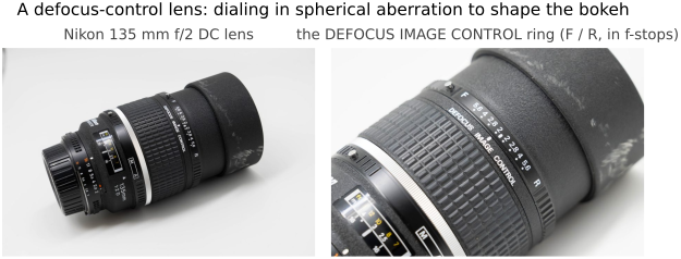
Some production lenses make this adjustable. The Nikon 135 mm f/2 DC ("Defocus Image Control") carries a second ring, marked in f-stops with an F and an R, that dials a controlled amount of under- or over-corrected spherical aberration into the lens, letting the photographer soften the foreground or the background bokeh on purpose (Figure 22.7.11). It is this section's principle built into a knob: the aberration is not a defect to remove but a parameter to set.
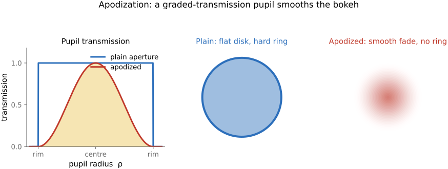
Apodization shapes the aperture's transmission rather than its geometry. An apodizing lens places a radially graded filter in or near the pupil, fully transparent at the center, smoothly darkening toward the edge, so the pupil has a soft, feathered rim instead of a hard cut-off. Because an out-of-focus highlight is the image of the pupil, softening the pupil's edge softens the defocus disk's edge: the bokeh disks lose their hard outline and their bright rim and become smooth, creamy gradients that melt into the background. This is PSF (point-spread function) shaping in hardware. It deliberately controls the blur profile and is the optical counterpart of computational bokeh, which shapes the same disk profile in software (cross-reference Chapter 23.1, Bokeh, focus stacking, and depth-of-field control). The cost is light: the graded filter dims the edge of the aperture, so an apodized lens transmits less than its f-number suggests (its T-stop is darker, from Chapter 22.1, Aberrations and optical challenges).
22.7.9 From shaped glass to thin structures: Fresnel, diffractive, GRIN, metalenses⧉
Everything to this point has been shaped glass, a bulk of transparent material whose curved surfaces refract the light. But a lens does only one essential thing: it imposes a particular delay (a phase profile) across the wavefront, bending the rays to a focus. If only the effect on the wavefront matters, then the bulk of the glass is wasted material, and a series of designs throw progressively more of it away. The recurring idea is to reproduce the required ray directions or wavefront with less conventional bulk. These are related constructions rather than one monotonic progression: a refracting Fresnel lens preserves facet slopes, a diffractive element can wrap phase, and GRIN optics use a volume index gradient. It starts with a lens you can hold (the Fresnel lens) and ends with one essentially without thickness at all (the metalens), the conceptual destination handed off to the flat-optics chapter in the Advanced part.
Fresnel lenses⧉
Look at where a lens actually bends light: only at its surfaces, and what matters there is the local slope of the surface, which sets the local refraction angle. The thick glass between the surfaces just adds delay and weight; two points on the lens at the same surface slope refract a ray the same way regardless of how much glass sits behind them. A Fresnel lens exploits exactly this. Slice the smooth lens profile into concentric annular zones and collapse each zone down to one thin sheet, keeping each zone's surface slope but discarding the bulk behind it. The smooth curve becomes a set of concentric sawtooth rings, a ring of tiny prisms, each prism reproducing the local refraction the original curve had at that radius. The bending is nearly the same, but the glass volume is much smaller.
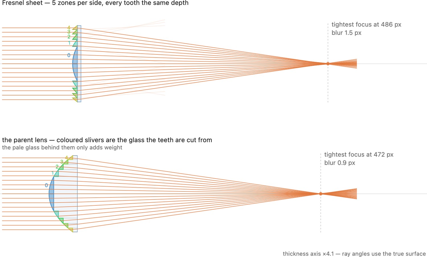
The main advantage is: a Fresnel lens is far thinner, lighter, and cheaper than the equivalent thick lens (it can be molded as a flat plastic sheet). The price is image quality. The sharp discontinuities between rings scatter and diffract light, and the ring structure itself is faintly visible as concentric artifacts, so Fresnel lenses are used wherever thinness, weight, or cost matters more than sharpness. The design dates to Augustin Fresnel, who devised it for lighthouses, which needed an enormous aperture to throw a beam to the horizon but could not use a single unliftable blob of glass (Figure 22.7.14). Today Fresnel lenses appear in condenser and projection optics, page and screen magnifiers, solar concentrators, vehicle brake lights and thin illumination optics, and, refined to high precision, in thin optical systems. The phase-Fresnel (PF) telephoto elements discussed next are specifically diffractive structures, not simply conventional refracting Fresnel facets.
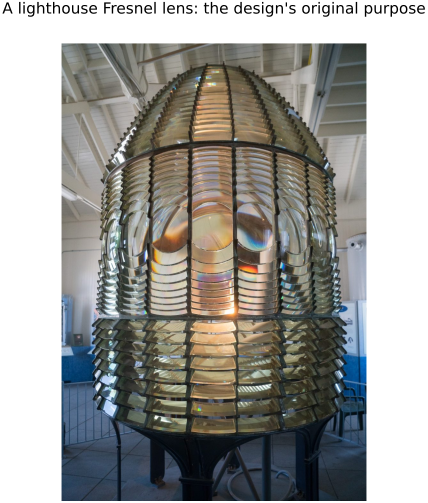
The Fresnel lens is the first step away from bulk shaped glass toward thin structured optics: it treats the lens as a thin structure that approximately preserves ray bending, without necessarily preserving the continuous phase of the original lens rather than as a solid of revolution. Follow that step further and you reach diffractive optics, then graded-index glass, and ultimately flat optics and metalenses, and the same "keep the phase, drop the thickness" idea reappears one more time in wavefront coding (Advanced part).
Diffractive elements⧉
If the rings are made much finer, down toward the scale of the wavelength of light, the element stops bending light mainly by refraction off prism facets and starts bending it by diffraction off a fine periodic structure. A diffractive optical element steers light by interference from its surface pattern, and it has a peculiar, valuable property: its dispersion has the opposite sign to glass. Ordinary glass bends blue more than red; a diffractive structure does the reverse. So pairing a diffractive element with a refractive one lets the two cancel each other's chromatic aberration, a hybrid lens that corrects color with far less weight and exotic glass than a stack of achromats would need. This is the principle behind Canon's DO (diffractive optics) and Nikon's PF (phase Fresnel) telephoto lenses: thin, light, and well-corrected for color, though still prone to flare at the ring structure under bright sources.
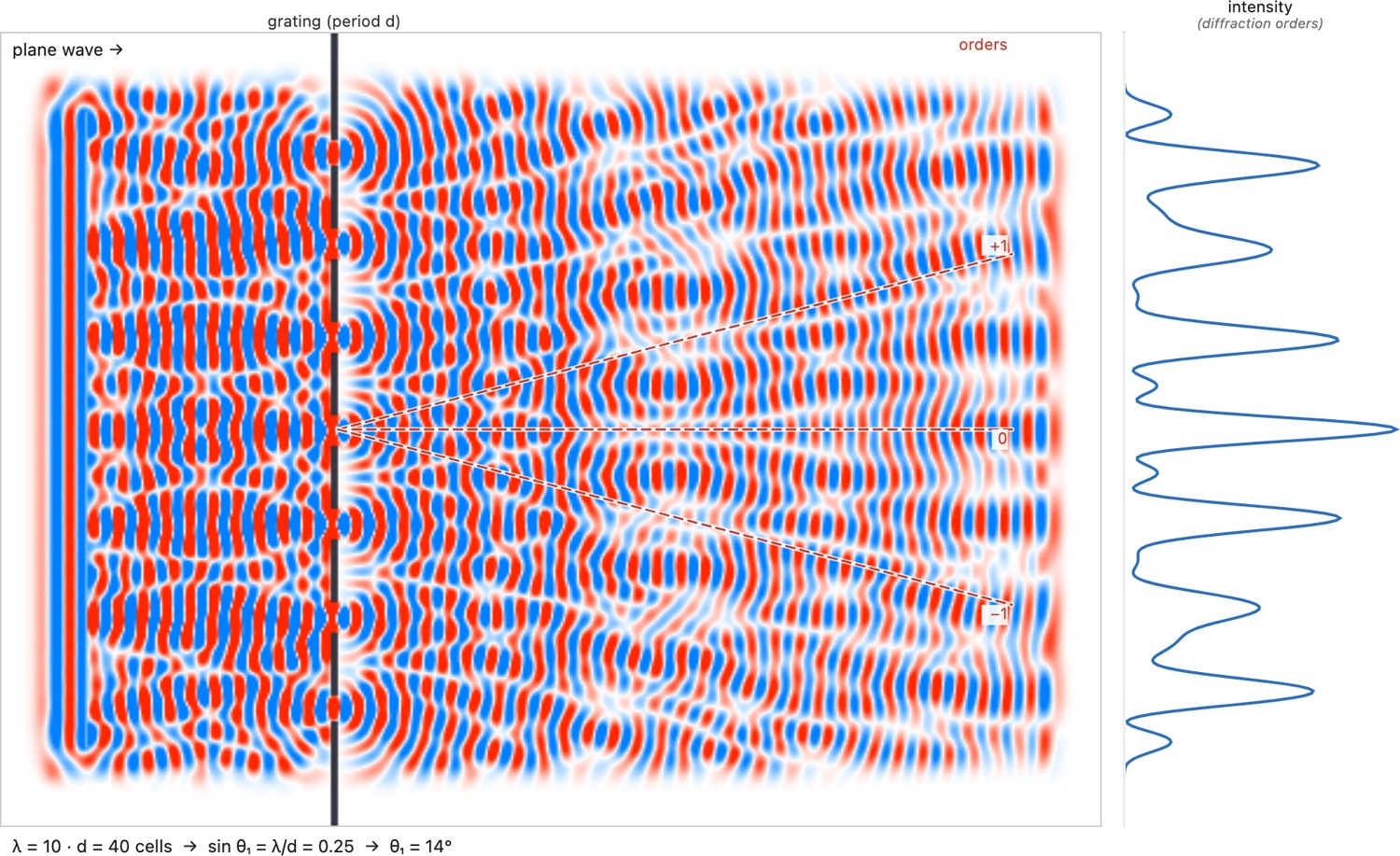
The canonical diffractive element is the diffraction grating, a periodic array of slits or grooves of period $d$. Wavelets from adjacent periods reinforce only where their path difference is a whole number of wavelengths, at normal incidence the grating equation $d\sin\theta_m = m\lambda$, so incident light splits into discrete orders $m = 0, \pm1, \pm2, \dots$ at angles $\theta_m$. Because $\theta_m$ grows with $\lambda$, a grating disperses white light into a spectrum (the heart of the spectrometer, and the rainbow sheen of a CD) dispersing in the opposite sense to a prism. This is the same opposite-sign dispersion that lets a diffractive element cancel a refractive one's chromatic aberration (Figure 22.7.15).
Mirrors (cross-link)⧉
Reflection is the other way to escape dispersion entirely: a mirror bends every wavelength identically and so adds zero chromatic error. That makes mirror-based designs a natural companion to the diffractive trick in this arc, and they were covered above under Mirrors: catadioptric and reflecting systems. See that section for the folded telephoto, the ring pupil and its doughnut bokeh, and the reflecting and catadioptric telescopes.
GRIN (gradient-index)⧉
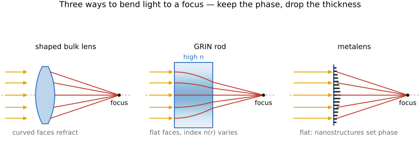
The designs so far bend light at surfaces. A gradient-index (GRIN) element bends it inside the material instead. Its refractive index is not constant but varies continuously through the glass, typically highest on the axis and falling toward the edge. Because rays curve toward higher index, a ray crossing such a medium follows a gently curved path rather than a straight one, and a slab with flat, parallel faces can therefore focus, with no curved surface at all. The bending is distributed through the volume rather than concentrated at a surface. Gradient-index optics show up in optical-fiber coupling, endoscopes, the rod-lens arrays in photocopiers and scanners, and, remarkably, in the lens of the human eye, which is gradient-index and uses exactly this trick to focus with gentle surfaces.
Metalenses (forward-ref)⧉
The endpoint of the arc keeps the phase profile and drops the thickness almost entirely. A metalens is a flat surface tiled with sub-wavelength nanostructures, a metasurface whose tiny pillars or fins each impose a chosen phase delay on the light passing through, so that the array as a whole reproduces a full lens's phase profile in a thin structured layer, usually on a supporting substrate. Its finite feature height, bandwidth, angular response, and efficiency remain design constraints. It is the logical limit of "keep the phase, drop the thickness": a lens with no curve and no bulk, just a patterned film. We place the metalens here as the conceptual destination of the Fresnel → diffractive → graded-index → flat-optics progression; its real workings (how the nanostructures are designed, how they handle color and efficiency, and how they fit into a computational camera) are the subject of the flat optics and metalenses chapter in the Advanced part (forward-reference).