18.6 Gradient-domain tone mapping⧉
The methods so far split the image into layers and recombine them. Gradient-domain tone mapping works on a different object: the derivatives of the image. It shrinks the large gradients, which carry the dynamic range, keeps the small ones, which carry the detail, and then solves for the image whose gradients are closest to the edited field. The operation is different in kind from a base/detail split, and it is the third member of the trilogy of Part 10, Edges matter: Poisson reconstruction works across edges, where the bilateral filter preserves them and seam optimization avoids them (Chapter 10.10, Recap: which edge-aware technique when?). This chapter presents the method, explains why it is harder to control than it first appears, and proposes a screened variant that ties its large scales to a simpler operator.
18.6.1 Attenuating large gradients: Fattal, Lischinski and Werman⧉
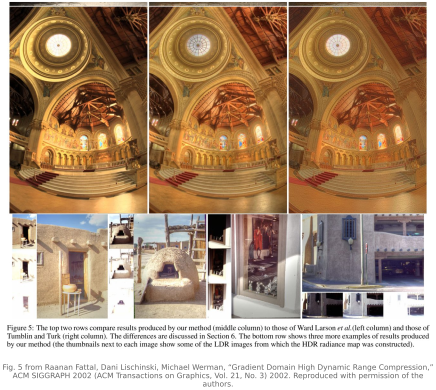
The method of Fattal, Lischinski and Werman starts from the log luminance $H=\log Y$ Fattal et al. 2002. A large gradient of $H$ is an edge with a large ratio across it, a window frame or the silhouette of a building against the sky; a small one is texture. The operator multiplies the gradient by an attenuation factor that is close to one for small gradients and falls for large ones,
with $\beta$ a little below one, around 0.85, and $\alpha$ a fraction of the average gradient magnitude, around a tenth. Gradients above $\alpha$ are reduced, those below it slightly enlarged. To decide what counts as a large edge at several scales, the published method computes the factor on a Gaussian pyramid of gradient magnitudes and combines the levels from coarse to fine, so a strong edge is recognized even where its fine-scale gradient is spread over several pixels.
The edited field $G$ is in general not the gradient of any image. The method therefore solves for the image $I$ whose gradient is closest to $G$ in the least-squares sense, which leads to the Poisson equation
with Neumann boundary conditions, solved with a multigrid method (Chapter 10.8, Poisson image editing). Exponentiating $I$ gives the compressed luminance, and color is put back as for any luminance operator (Chapter 18.2, Global tone mapping).
18.6.2 Why it is hard to control⧉
The method rarely produces the halos of a blurred base, since it never blurs across an edge. Its difficulties are of another kind.
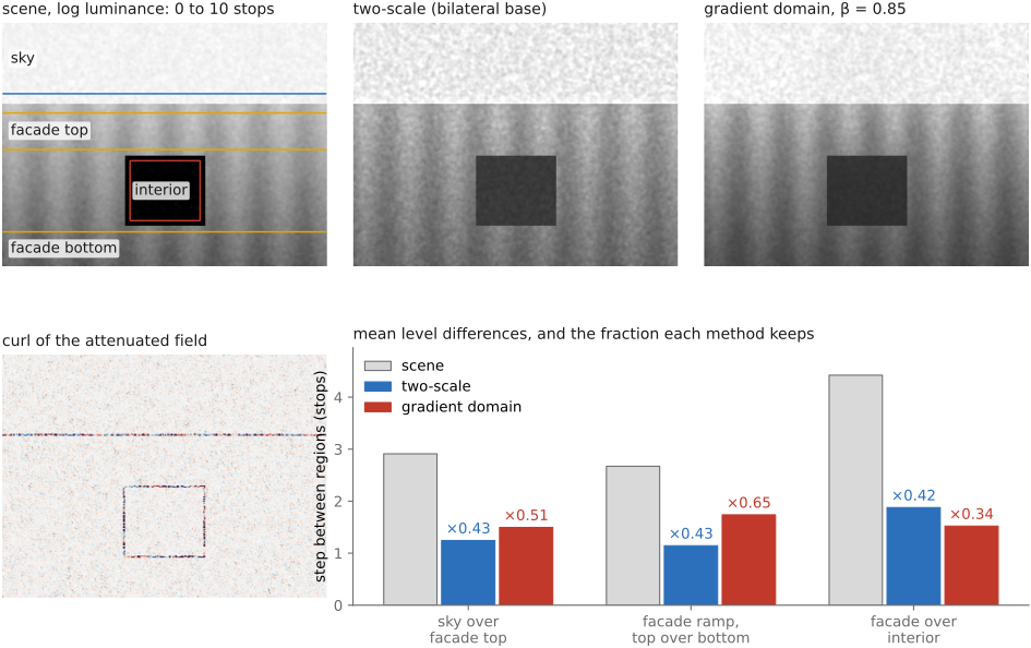
The edited field is not integrable. Attenuating gradients by a factor that varies across the image breaks the consistency of derivatives: the sum of the edited gradients around a closed loop is no longer zero. The least-squares solve resolves the inconsistency by spreading the error over the whole image, and it spreads it into the lowest frequencies, where it is least visible locally and most damaging globally. Regions drift toward one another, and unevenly: on a synthetic sky above a facade, a two-scale operator keeps about 0.43 of every step between regions, while the Poisson solve keeps 0.34 of a sharp 4.4-stop step at a window and 0.65 of a slow 2.7-stop ramp across the facade, and on some real scenes the large regions change order, as Figure 18.6.3 shows on the vine sunset. The large-scale relationships of the scene, which Chapter 18.1, Tone mapping and perception argues the viewer reads, are exactly what the method does not control (Figure 18.6.2).
The solve is global. Changing a gradient at one place moves the reconstructed values everywhere, so the method has no local control and its parameters act in ways that are hard to predict; small changes of $\alpha$ or $\beta$ can change the overall rendering. It also has no direct control over the output's levels or histogram.
The boundary and mean constraints are especially visible on a flat patch. Gradients describe changes within the patch, so adding a constant to log luminance leaves those gradients unchanged. An anchor is required to choose an overall level. After attenuating gradients, the reconstruction also has to reconcile modified derivatives that may not integrate to one exact image. Fixing the mean removes the additive ambiguity, but does not independently specify every part of the output histogram. This is why a gradient-domain reconstruction may still benefit from a subsequent tone curve: the reconstruction fits spatial differences, while the curve offers direct control over the rendered distribution of values.
And noise is treated as detail. Small gradients are kept or slightly enlarged while large ones shrink, so in flat dark regions, where the gradients are mostly noise, the noise keeps its strength while the scene's contrast falls around it. Later work moved the processing to a perceptual measure of contrast at several scales, which handles some of these issues Mantiuk, Myszkowski & Seidel 2006, but the low-frequency drift is inherent to reconstructing an image from a non-integrable field.
18.6.3 A screened version: anchoring the large scales⧉
The drift suggests a remedy. The gradient field is trustworthy at fine scales, where it carries the detail, and untrustworthy at coarse ones, where its inconsistencies accumulate. A simple operator is the reverse: a two-scale tone map computed at low resolution gets the large-scale relationships right, since it has no non-integrable field to reconcile, and lacks only detail (Chapter 18.3, Two-scale and bilateral tone mapping). We can combine the two by asking the solution to follow the edited gradients and, weakly, a coarse anchor $b$:
Here $G$ is the attenuated field of Fattal and colleagues, $b$ is the log luminance of a bilateral two-scale tone map computed on a downsampled copy of the radiance map and upsampled, and $\lambda$ sets the strength of the anchor. Setting the derivative to zero gives the screened Poisson equation
which, unlike the plain Poisson equation, has a unique solution without any boundary or mean constraint, and can be solved in one pass with a fast Fourier or cosine transform Bhat et al. 2008 (screened Poisson). In the Fourier domain, at spatial frequency $\omega$,
so the solution takes its low frequencies, below $|\omega|\approx\sqrt\lambda$, from the anchor and its high frequencies from the integrated gradients. The constant $\lambda$ is therefore a spatial scale: structures larger than about $1/\sqrt\lambda$ pixels follow the simple operator, smaller ones follow the gradient field. At $\lambda=0$ the method is Fattal's; as $\lambda$ grows it becomes the anchor. Because the anchor fixes the large scales, the drift cannot accumulate beyond that size, the overall levels are set by the anchor rather than by an arbitrary constant, and the gradient attenuation only has to do what it does well, compressing edges while keeping detail.
screened_gradient_tonemap(Y, lam, alpha, beta, anchor_scale=1/8):
    H = log(max(Y, eps))
    G = fattal_attenuation(grad(H), alpha, beta)          # multiscale factor Phi times grad H
    small = downsample(Y, anchor_scale)
    b = upsample(log(two_scale_tonemap(small)), size(Y))  # coarse but trustworthy rendering
    rhs = lam * b - div(G)
    u = solve_screened_poisson(lam, rhs)                  # DCT: divide by lam + eigenvalues of -Laplacian
    return exp(u)                                         # then color ratios and display encoding
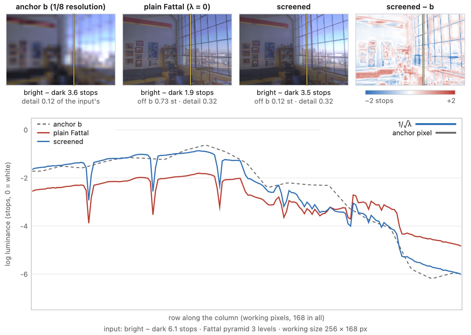
This is an experiment rather than a published operator, and Figure 18.6.3 lets the reader run it. Run on the book's radiance maps, it does what the analysis suggests for the large scales. On the office scene, the difference between the brightest and darkest regions is 6.07 stops in the input, 3.64 in the anchor and 1.90 after the plain Poisson solve, which has drifted; screening brings it back to 2.37, 3.20, 3.49 and 3.60 stops as the crossover $1/\sqrt\lambda$ shrinks from 100 to 32, 16 and 8 pixels. On the vine sunset, the plain solve swaps the order of large regions four times among the brightness deciles, and screening restores it. The fine texture stays the gradient method's until the crossover is a few pixels wide.
The edges behave differently from the prediction. There is no overshoot. The solution is the plain result plus a low-pass of the anchor's difference from it, so at each strong edge the difference between the two operators' steps is spread over about $1/\sqrt\lambda$ on each side: the bright side is darkened and the dark side lifted near the edge, a soft ramp of the opposite sign to a blurred-base halo. A full-resolution anchor gives about the same ramp, so it comes from the crossover, not from the anchor's coarse resolution, whose blur shows only once $1/\sqrt\lambda$ is as small as one anchor pixel. And the method inherits one weakness from Fattal's: at its default parameters, the gradient attenuation keeps only a third to two fifths of the input's texture contrast, where a full-resolution two-scale map keeps 70 to 95%. Whether it beats the two-scale operator alone is a question for the evaluation methods of Chapter 18.11, Evaluating tone mapping.