14.1 What can super-resolution actually do?⧉
Take a photograph, throw away three quarters of its pixels, and ask an algorithm to put them back. Two very different things could be happening.
A small character can have several sharp explanations after blur and sampling. Figure 14.1.1 exaggerates the demand for a unique answer from insufficient measurements.
Different sub-pixel offsets can separate some aliased components by supplying additional equations. This is the basis of Chapter 14.2, Multi-frame super-resolution. Accuracy depends on the optical transfer, sampling coverage, noise and registration; additional frames do not guarantee a correct reconstruction.
With one photograph, several high-resolution images can fit the same measurements. Interpolation assumes a form of smoothness or band limitation; learned methods use regularities fitted from training images. These assumptions can improve accuracy on appropriate scenes, but cannot establish the identity of unresolved detail in every case.
Both can be checked against a suitable higher-resolution reference or an independent capture. Without one, agreement with the observed image checks consistency, not uniqueness.
14.1.1 What the sensor kept and what it folded⧉
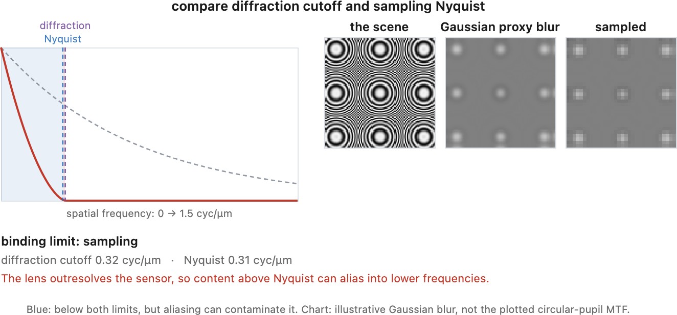
A sensor samples the image formed by the lens on a grid of pitch $\Delta$. Sampling theory says a signal band-limited below the Nyquist frequency $1/(2\Delta)$ is recoverable exactly from those samples, and that content above it is not lost quietly: it is folded down and added to the low frequencies, where it is indistinguishable from real low-frequency content. That folding is aliasing, and in photographs it looks like moire on fabric, stair-stepped diagonals, and false detail in foliage.
Aliased content contributes to the samples, mixed with other frequencies. Content suppressed to zero before sampling contributes nothing. For ideal diffraction-limited incoherent imaging at wavelength $\lambda$, the optical cutoff is approximately $1/(\lambda N)$ cycles per unit length in the sensor plane, with $N$ the image-side f-number approximation used here. Pixel integration adds its own transfer function and possible zeros. Real contrast and noise can impose a useful resolution limit well below the optical cutoff.
Additional sampling helps where the optics and pixel aperture transmit detail that the sensor grid undersamples. Sensor size alone does not determine that regime: compare pixel pitch, aperture, aberrations and noise. No number of ordinary shifted captures restores a component suppressed in every measurement.
14.1.2 The forward model, and why this is an inverse problem⧉
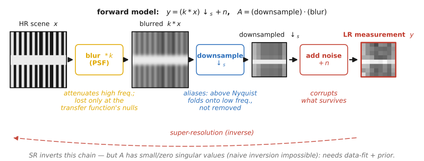
Write down what the camera did. A high-resolution image $x$ is blurred by the optics and the pixel aperture, sampled on the sensor grid, and corrupted by noise:
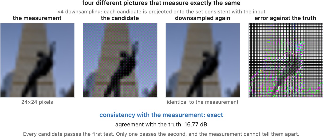
with $B$ the blur and $S$ the downsampling. Super-resolution is the recovery of $x$ from $y$, which is the same shape of problem as everything in Part 13, Denoising and Chapter 16.2, Non-blind deconvolution, with a harder operator. It is ill-posed in the strict sense: $S$ maps many different $x$ to the same $y$, so the data cannot choose between them and something else must (Figure 14.1.3, Figure 14.1.4).
A regularizer or learned prior selects among weakly constrained images. Its influence depends on signal-to-noise ratio and the operator, even in denoising. At fourfold enlargement per dimension there are sixteen unknown output samples per input sample in a scalar model. This counts equations and unknowns; it does not assign a percentage of the finished photograph to invention.
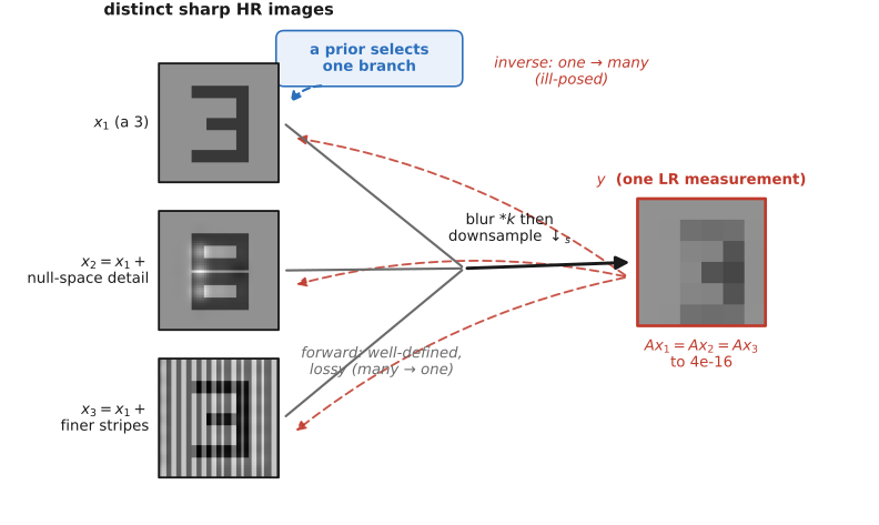
3, an 8, and a fence pattern) stand for images that blur-then-downsample cannot tell apart, all producing the same low-resolution $y$ because what distinguishes them is exactly what the forward model removes. The forward arrow is well defined and lossy; the backward arrow is one-to-many. The panels are a schematic of that situation rather than a computed example: images that truly share a measurement differ only by components in the forward operator's null space. The data cannot choose among such preimages; only a prior can.The practical reading of $y = SBx + n$ is that the three parts fail differently and must be handled separately. Get $B$ wrong and the result is soft or ringing. Get $S$ wrong, which is what happens when a method trained on clean downsampling meets a real photograph, and the result is confidently wrong, which Chapter 14.9, Blind and real-world super-resolution is about. Ignore $n$ and the method amplifies noise into texture, which is the failure mode that looks most like success.
14.1.3 Two operations, one word⧉
Reconstruction methods can use measured sampling diversity, image priors, or both. With known shifts and adequate coverage, a burst constrains detail that one frame cannot distinguish. Unreliable alignment and nearly suppressed frequencies still require regularization. Single-image methods exploit assumptions about edges, repeated patches or training-image statistics. Their inferred detail can be correct, but its correctness does not follow from appearance alone.
Baker and Kanade (Baker & Kanade 2002 (limits of super-resolution)) and Lin and Shum (Lin & Shum 2004 (fundamental limits)) analyze limits under specified imaging and noise assumptions. A roughly twofold gain is a useful practical scale in some systems, not a universal cutoff or guarantee. Distinguish requested output enlargement from measured resolving power.
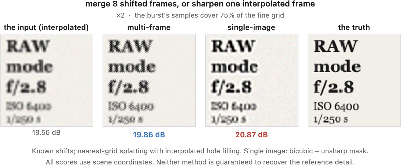
Additional captures can constrain unresolved detail. An image prior can select plausible detail. A reconstruction may use both, and visual sharpness alone does not show which details are accurate.
14.1.4 What a resolution number means once a prior is involved⧉
A fourfold enlargement conventionally means four times the width and height, or sixteen times the pixel count; always state the convention. Resolved detail is a separate measurement. It can vary across one photograph because of blur, texture, motion and local sampling coverage. Picture a 4× enlargement of a portrait taken in front of a brick wall with a sign. The regular brick texture is easy for a prior to extend convincingly, and errors there matter little. The letters on the sign are constrained by what letters look like, but a wrong guess changes the word. The face is where a prior has the most to offer and where a plausible invention is least acceptable, since it can change who the person appears to be. One output, one scale factor, and three different answers to how much of the detail was measured.
Report errors on fine structures as well as whole-image averages. Chapter 14.6, The perception-distortion tradeoff and perceptual super-resolution distinguishes expected reconstruction error from output-distribution realism. Neither PSNR nor apparent crispness measures every aspect of resolution.
Recap: big lessons of this chapter
Additional captures can constrain unresolved detail. An image prior can select plausible detail. A reconstruction may use both, and visual sharpness alone does not show which details are accurate.