16.5 Spatially varying blur⧉
A point near the image center and one near a corner can trace different paths during the same exposure. Modeling those paths independently wastes the constraint that one camera produced them. A physical motion model derives their relationship and provides a forward operator that can be evaluated without storing a full blur matrix.
16.5.1 Rotational camera shake⧉
Everything above assumed a single kernel convolved over the whole image, shift-invariant blur, where the squiggle is the same in every corner. That assumption is the foundation of the FFT trick and of "the kernel" as one small object. And real camera shake violates it.
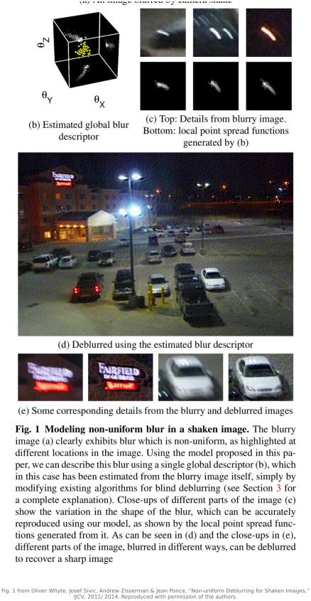
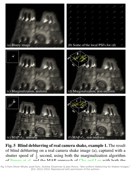
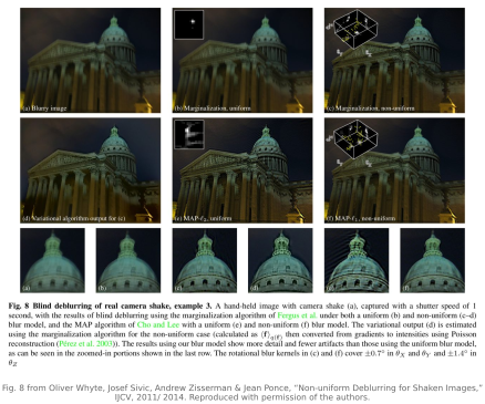
Camera rotation generally induces a position-dependent image motion. Pure roll around the optical axis leaves the center fixed and moves outer points along arcs. Pitch and yaw also move the center; they do not generally produce a motion field that vanishes there. A small field of view may admit a translation approximation. The spatially varying example in Figure 16.5.4 illustrates why the rotation model matters.
Depth-dependent defocus, lens aberrations and independently moving objects also create spatial variation. Translational camera motion is itself depth-dependent in a general 3-D scene. A known geometry and visibility model can still define a linear map from latent radiance to measurements; estimating that geometry makes the full problem harder.
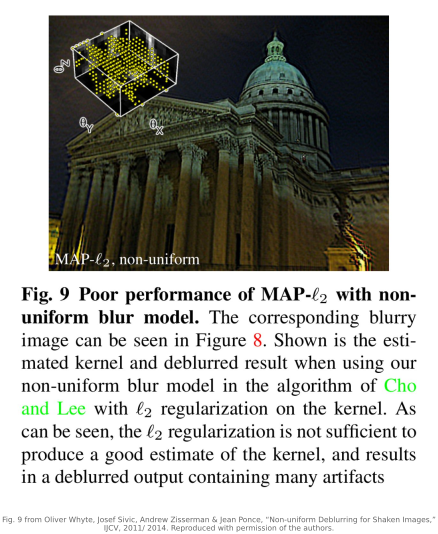
The better model (Whyte, Sivic, Zisserman & Ponce, 2011/2014 Whyte et al. 2011/2014) does not try to write down a different kernel at every pixel independently: that would be hopelessly many unknowns. Instead it goes back to the physics: the blurry image is a weighted sum of the sharp image seen under many camera poses, integrated over the camera's rotational trajectory during the exposure. The unknown is that trajectory (a path through the low-dimensional space of camera rotations) and it is one underlying 3-D motion. From it, the spatially-varying PSF at every pixel is derived, automatically consistent across the frame because it comes from a single physical cause. Far fewer unknowns than an independent kernel per pixel, and physically meaningful ones.
For pure rotation and a static scene, use the calibrated projection $H_j=C R_j C^{-1}$ for each exposure sample, with camera intrinsics $C$ and relative rotation $R_j$. A discrete exposure model is
Each $\mathcal W_j$ backward-samples the reference image into the exposure view using consistent coordinates. Its adjoint scatters interpolation weights, including boundary handling; it is generally not an inverse warp. A static blur exposure constrains pose occupancy, not necessarily the chronological order in which those poses occurred.
The consequence for the math is that deblurring becomes inversion of a global, non-stationary linear operator (the pose-integral) rather than a convolution. It is still linear in $X$, and it is still the same data-fit + sparse-prior recipe; what changes is that the forward operator no longer diagonalizes in Fourier, so there is no single-FFT trick (L6.8 does not apply when the operator is not a convolution). We are back to the matrix-free iterative solvers of the previous chapter (conjugate gradient and friends) applying the pose-integral operator and its transpose at each step. A further wrinkle that Whyte et al. 2014 handles and that any "realistic" deblurring must face: real shots have saturated highlights (a streetlamp clips to pure white), and clipping is a non-linearity that breaks the linear convolution model outright: handling those saturated pixels specially is part of making the method work on actual photographs.
16.5.2 A table of blurs, and which are convolutions⧉
Summarize the blurs in one place, because the single most consequential property of any blur is whether it is shift-invariant (one kernel convolved everywhere, the only case the FFT/Wiener machinery handles directly) or spatially varying, where it is not a convolution at all. With Oliver Whyte's camera-shake model as the centerpiece, the catalog is:
| blur source | physical cause | shift-invariant? |
|---|---|---|
| Translational camera motion | the camera slides sideways during the exposure | approximately for constant depth and suitable motion; depth variation causes parallax |
| Camera shake (rotation) | wrist pitch/yaw, the dominant hand tremor | generally spatially varying; pure roll has a stationary center (Whyte et al. 2011/2014) |
| Defocus | a point's depth differs from the focus plane | approximately uniform on a single depth plane; varying depth and occlusion require more |
| Subject / object motion | something in the scene moves while the camera is still | no, only the moving region blurs, each along its own path |
| Lens aberrations | imperfect optics: coma, astigmatism, field curvature | no, mild on-axis, worse toward the field edge; per-channel for chromatic aberration |
| Atmospheric turbulence | hot air, long lenses | no, a shimmering warp that varies in space and time |
Whether convolution is adequate depends on the scene and regime. A frontoparallel constant-depth plane under lateral translation can give a uniform motion blur; one defocus depth with approximately field-invariant optics can also give a convolution. General 3-D translation, varying depth and visibility require more.
16.5.3 What ships in a phone⧉
Polyblur estimates mild blur and applies a polynomial approximation to its inverse (Delbracio et al. 2021). Repeated blurs can be combined to approximate correction without a direct Fourier division. The approximation has a limited useful regime and still needs noise/artifact control. Deblurring has also reached consumer photo software. Google's Photo Unblur (2022) sharpens existing photographs, including scans of old prints, and its earlier Face Unblur (2021) used a simultaneous capture from a second camera to sharpen faces in motion. Their implementations are not published, so they illustrate the application rather than any particular algorithm; the specific published algorithm is the relevant unit of comparison here.
Coded apertures and wavefront coding alter the forward response to improve identifiability or conditioning over a designed range (Dowski & Cathey 1995). They still trade light, noise and resolution; no optical design makes every frequency recoverable. See Chapter 33.3, Coded aperture and Chapter 33.1, Wavefront coding.
A simple polynomial example explains how additional blurring can approximate an inverse. Write a mild blur as $B=I-E$. When the spectral radius of $E$ is less than one, $B^{-1}=I+E+E^2+\cdots$. Truncating after the quadratic term gives $I+(I-B)+(I-B)^2=3I-3B+B^2$: combine the input, one reblurred copy and a twice-reblurred copy with signed weights. This is an illustrative inverse polynomial, not the complete Polyblur algorithm or its fitted coefficients. Severe attenuation makes the approximation poor, and noise still requires control. The implementation advantage is that applying a few local blurs can be cheaper than solving a large blind reconstruction.