15.11 Synthetic data, unprocessing, and raw reconstruction⧉
Raw-domain training needs representative targets and corruption. Capturing low-noise references often requires repeated static exposures and calibration; motion and changing light complicate the pairs. Chapter 13.2, Denoising by averaging explains why an averaged reference remains an estimate.
Finished photographs are plentiful, but are not all clean or camera-linear. Unprocessing approximately reverses selected rendering operations to make synthetic camera-domain training data.
Brooks et al. demonstrate this approach for learned raw denoising (Brooks et al. 2019 (Unprocessing)).
15.11.1 The inversion, step by step⧉
Take an sRGB photograph and walk the pipeline backwards, undoing each stage in reverse order.
Undo the display encoding. Decode the stated sRGB transfer function. This reverses that encoding on represented values; it does not reverse an unknown tone map, clipping or compression.
Undo an assumed tone curve. The actual camera curve may be unknown, local or noninvertible where clipped. A monotone curve with very small slope also amplifies quantization on inversion. Unprocessing uses a chosen approximate family whose effect should be validated on the target data.
Undo a sampled or known color matrix and white-balance gains in the correct order. A nonsingular matrix and nonzero gains are invertible before clipping, but may be poorly conditioned. Values reconstructed from clipped colors are inferred, not recovered measurements.
Remosaic. Keep one channel per pixel according to the array, discarding the rest. This one is exact, since it is the forward model of Chapter 15.6, Learned demosaicking.
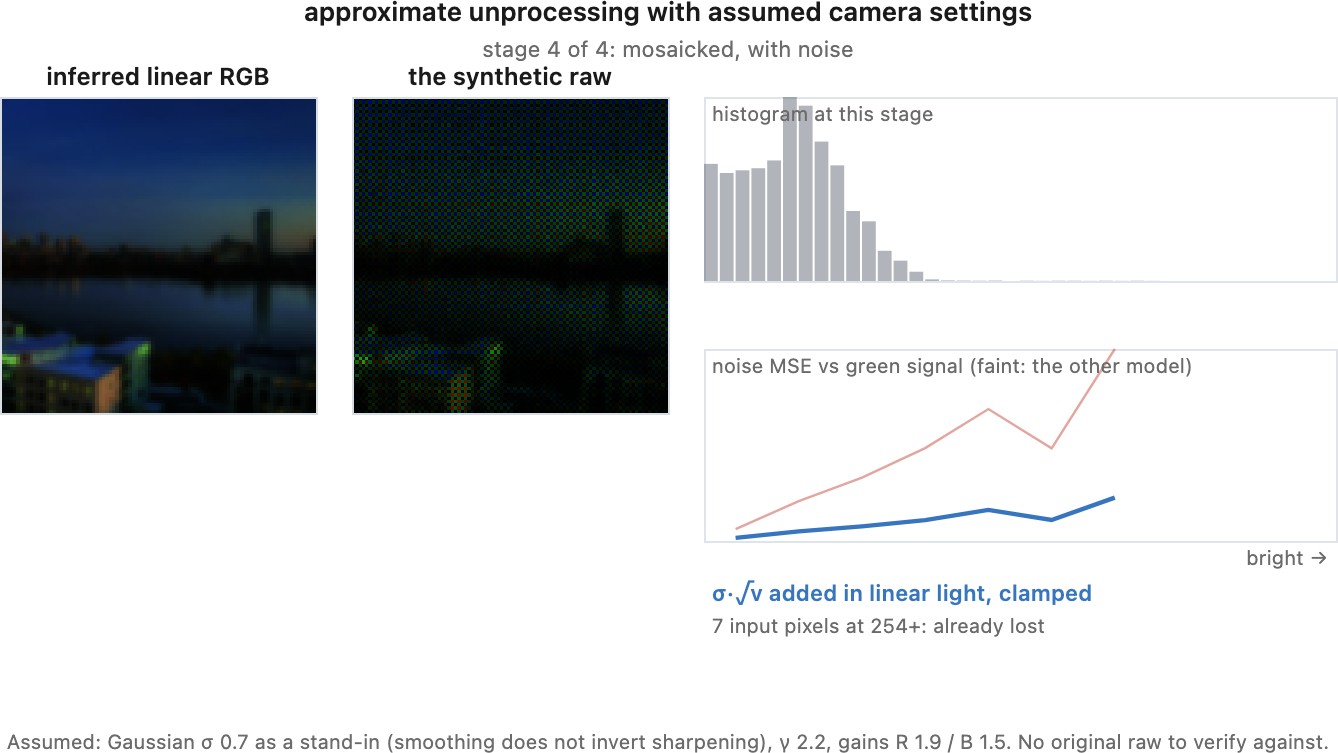
Add noise after converting to a calibrated linear camera domain and applying the CFA. Sample compatible shot/read-noise parameters, with correlations or clipping included when required by the target sensor. A Gaussian approximation with affine variance does not exactly reproduce every raw-noise distribution.
# unprocessing: sRGB photograph -> synthetic noisy raw
lin   = decode_srgb(img)              # display encoding -> linear
lin   = inverse_tone_curve(lin)             # the camera's S-curve, approximately
cam   = inverse_color_matrix(lin, ccm)      # sRGB -> camera RGB
cam   = safe_inverse_gains(cam, white_balance_gains)           # specify highlight handling; simple division is insufficient at clipping
mosaic= apply_bayer(cam)                    # keep one channel per pixel
a, b  = sample_noise_params()               # a real sensor's range of gains
raw   = mosaic + sample_noise(mosaic, a, b) # LINEAR domain: the model holds here
15.11.2 Why an approximate inverse is good enough⧉
Several of those steps are only approximately invertible, and the true parameters of the camera that took the photograph are unknown. It would be reasonable to expect the synthetic raws to be wrong in ways that mislead the training.
Approximate unprocessing can still improve training when it makes the distribution more representative than adding white noise directly to encoded RGB. That is an empirical result, not an invariance to an incorrect tone curve. The joint distribution of clean values, noise, color and structure can change under each approximation.
Brooks et al. report strong real-noise benchmark results under their processing/unprocessing and training choices. Evaluate each component and cross-camera generalization before assuming the same gain for another pipeline.
The limitation is the one the previous paragraph implies. Anything the finished photograph no longer contains cannot be reconstructed: clipped highlights, detail already destroyed by the original camera's denoiser, and the artifacts of the original demosaicker, which are now baked in as if they were scene content. Training on unprocessed data therefore teaches a network to reproduce some of another pipeline's mistakes.
15.11.3 Raw reconstruction as a goal of its own⧉
The same inversion, done carefully, is useful for its own sake. A photographer with only a JPEG has lost the editing latitude a raw file carries; recovering a plausible raw restores some of it, and there is a line of work on doing this well, either by fitting the specific camera's pipeline or by storing a small amount of metadata alongside the JPEG at capture time to constrain the reconstruction.
Unprocessing aims to create useful training examples. Raw reconstruction aims to estimate a particular capture, often to support editing. A plausible linear representation can make adjustments more convenient, but it does not restore clipped photons or lost scene detail. Additional stored metadata can constrain inversion; it does not make arbitrary JPEG processing exactly reversible.
15.11.4 The pipeline diagram, walked backwards⧉
Keep each intermediate labeled: encoded sRGB, decoded RGB after the camera's tone rendering, an approximate untone-mapped linear representation, camera RGB and a camera mosaic. Record every assumed matrix, gain, noise parameter and clipping rule. This permits unit and ordering checks, especially before noise injection.
The order can be checked with a simple noise experiment. Start from an approximately linear camera-space signal, add sensor noise there, and then apply white balance and the color matrix. White balance scales the variances differently by channel, and the matrix can introduce cross-channel covariance. Adding independent noise after those operations creates a different training problem, even if the displayed grain looks similar. Likewise, treating a clipped display value as an invertible measurement invents a certainty that the original exposure did not contain. Track the space and the uncertainty at each inversion step, rather than viewing unprocessing as a sequence of cosmetic adjustments.
This is a practical use of the color part's insistence on named spaces and encodings. A value's type tells us which inverse may act on it and where a sensor-noise model makes sense. Labeling those intermediate representations makes an ordering error visible before training a network, rather than leaving it to appear later as an unexplained failure on real raw data.