4.0 COLOR SPACES AND COLOR TECHNOLOGY⧉
Part 3, Visual perception and color established what color is to an observer: a spectrum reduced to three cone responses and then processed by the visual system. That reduction makes reproduction possible. A display can match a light without reproducing its spectrum, provided the match lies within the display's gamut and we specify the observer and viewing conditions.
A camera measures light through its own spectral sensitivities, which need not match the observer's. A display emits mixtures of its primaries. Color technology connects these devices using standardized measurements, conversion rules, and viewing assumptions. We have to separate what was measured from how it will be shown. The history of color science often joins those questions, because the experiments that established color measurement were themselves reproduction experiments. That connection explains much of the terminology and some of the awkwardness of photographic pipelines.
Chapter 4.1, Linear color reproduction and CIE XYZ develops the measurement and reproduction equations. Chapter 4.2, White balance and white point separates corrections for scene illumination from the reference white of an encoding. Chapter 4.3, Encoding: linear, gamma or log and Chapter 4.4, RGB color spaces explain how color coordinates become stored values. The remaining chapters cover perceptual coordinates, sensor designs, displays and printing, and the managed path from a file to an output device.
The section Encoding: linear, gamma or log#Color and encoding in real pipelines compares what real implementations do: where raw editors change coordinates, why OpenCV's panorama and HDR examples treat camera response differently, how Hugin and Enfuse pursue different objectives, and what deblurring and rendering require from their inputs. These implementation choices are part of understanding color, not details to postpone until an ISP chapter.
Chapter 4.9, Color TLDR gives the practical decisions: identify the input, choose a suitable working representation, and export with enough information for the next application to interpret it.
An RGB triple needs a color-space definition and a transfer function. Processing also needs its scale and image state: camera measurements, scene-referred values, and display-referred values support different operations. Preserve this information alongside the array. A floating-point data type alone does not tell you whether the values are linear or what their primaries are.
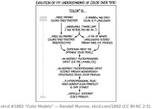
Figure 4.0.1 offers a less restrained introduction to the terminology.
Contents of this part
- 4.1 Linear color reproduction and CIE XYZ
- 4.2 White balance and white point
- 4.2.1 Von Kries adaptation and white balance
- 4.2.2 How do you know the illuminant?
- 4.2.3 White balance with mixed illuminant
- 4.2.4 White point in color space definitions
- 4.2.5 Spectral sharpening within LMS space
- 4.2.6 The limits of white balance, and CRI (color rendering index)
- 4.2.7 Spectral sharpening with general spectra
- 4.2.8 Subjective white balance
- 4.2.9 White balance datasets
- 4.3 Encoding: linear, gamma or log
- 4.3.1 Gamma encoding
- 4.3.2 Gamma the contrast operator (gamma adjustment)
- 4.3.3 System gamma: the end-to-end curve
- 4.3.4 Log encoding
- 4.3.5 PQ, the perceptual quantizer
- 4.3.6 HDR encoding
- 4.3.7 When to work on encoded values
- 4.3.8 Color and encoding in real pipelines
- 4.3.9 What gamma buys, and what it costs
- 4.4 RGB color spaces
- 4.5 Advanced color: opponents, perceptually-uniform, and preferred
- 4.5.1 Opponent color spaces and separating luminance and chrominance
- 4.5.2 Tensions: linearity, gamma, and opponents
- 4.5.3 HSV, HSL, and cylindrical color spaces
- 4.5.4 Perceptually uniform color spaces
- 4.5.5 Recap: a zoo of color spaces
- 4.5.6 Color appearance models
- 4.5.7 Preferred colors: skin, sky, and other memory colors
- 4.5.8 Color names and the prototypes behind them
- 4.6 Sensing color: multiplexing strategies
- 4.6.1 Multiplexing in time
- 4.6.2 Multiplexing in space: the color filter array
- 4.6.3 Multiplexing across separate sensors: the beam-splitter
- 4.6.4 Multiplexing per pixel by dispersion: color routers and nano-prisms
- 4.6.5 Multiplexing per pixel by tunable absorbers: quantum dots
- 4.6.6 Multiplexing in depth: stacked photodiodes
- 4.6.7 Hybrid strategies
- 4.6.8 Beyond trichromatic capture: full spectrum and multispectral
- 4.6.9 Spectral sensitivity: matching the eye, catching photons, and white balance
- 4.7 Synthesizing color
- 4.8 Recap: the full color pipeline, color management and ICC
- 4.9 Color TLDR
- 4.9.1 Physical color
- 4.9.2 Cones, LMS, and metamerism
- 4.9.3 Light and chromatic adaptation
- 4.9.4 XYZ
- 4.9.5 Chromaticity and gamut
- 4.9.6 Linear RGB, and why there are many
- 4.9.7 White balance and white point
- 4.9.8 Gamma is for encoding (and doesn't hurt processing much)
- 4.9.9 sRGB
- 4.9.10 RAW files
- 4.9.11 Log is for high dynamic range, video, and some processing
- 4.9.12 Opponent (luma-chroma) spaces
- 4.9.13 HSV is for UI
- 4.9.14 Perceptually uniform spaces are for differences
- 4.9.15 The full chain: from physical color to perceptual color to color names and memory
- 4.9.16 Color and encoding in the real world
- 4.9.17 What color space and encoding to do what?
- 4.10 Color terms
- 4.10.1 Radiometry: physical light, no observer
- 4.10.2 Photometry: physical light weighted by the eye
- 4.10.3 Colorimetry: color via the standard observer
- 4.10.4 Color appearance: perceptual, observer-dependent
- 4.10.5 Color spaces and encoding
- 4.10.6 Chronic confusions, named
- 4.10.7 One word, several meanings