19.4 Matting🔗⧉

A soft matte must preserve hair and motion-blurred edges while removing the old background. The observed color alone rarely specifies that separation. User constraints, extra captures and learned or explicit image models supply additional information.

19.4.1 The fundamental matting equation🔗⧉

We met the model already as the forward over operator; read backward, it is the matting problem. You see only the photograph, the observed color $C$ at each pixel, three numbers (R, G, B), and you must recover the foreground color $F$ (three numbers), the background color $B$ (three numbers), and the coverage $\alpha$ (one number) that produced it:

There are seven unknown scalar values and three observed channels at each pixel. This explains the ambiguity, but not how difficult every formulation must be: constraints and parameterization determine the numerical problem.

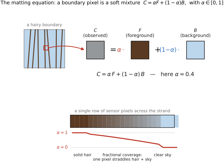
Extra information can be a controlled background, a trimap, local color assumptions or training data. Each constrains a different aspect of the ambiguity.

A trimap marks definite foreground, definite background and unknown pixels. The unknown region must include all mixed or uncertain pixels, which can cover a large area for smoke, translucent material or motion blur. Erode foreground and background masks to create a conservative band, then inspect it. A wrong hard constraint can prevent any later solver from recovering the correct matte.

A trimap provides reliable endpoints rather than solving every mixed pixel directly. Well inside an opaque foreground object, the observed color is a sample of foreground appearance; well outside, it is a sample of background appearance. Near a hair or a blurred boundary, neither is observed separately. The algorithm borrows information from the known regions and its image model to explain that mixture. Making the unknown band too narrow incorrectly labels mixed pixels as certain, so no later solver can recover the intended edge while honoring those labels. Making it wider leaves more uncertainty to the model. A good trimap is conservative about certainty, especially for motion blur, transparency, and fine hair.

19.4.2 Traditional matting approaches🔗⧉

When the only extra information is a trimap and a prior (no green screen) we are in natural-image matting: pull a soft matte out of an ordinary photograph against an ordinary, cluttered background. The field is now dominated by learning, and the two classical methods below survive less as production tools than as the clearest way to feel how hard the problem is and where the leverage comes from.

Bayesian matting (Chuang et al. 2001) is the brute-force answer, instructive because it shows how genuinely ambiguous the problem is. It attacks the unknown band pixel by pixel, working outward from the known regions. For each unknown pixel it gathers nearby known foreground and background colors, models each set as a Gaussian color cluster, and finds the $(F,B,\alpha)$ that best explains the observed $C$ in a maximum-a-posteriori sense, the likeliest mixture given the local color statistics. Sweep this from the trimap boundary inward and the band fills in. The instructive thing is how much modeling it takes to pin down one pixel: you must propose candidate foreground and background colors, weigh them by likelihood, and still the matte comes out noisy where the colors are ambiguous, because each pixel is solved on its own and neighboring alphas have no built-in reason to agree. Bayesian matting is the chapter's reminder that the seven-unknowns problem really is as ill-posed as it looks.

Closed-form matting eliminates local affine color-model coefficients to obtain a quadratic energy in alpha (Levin et al. 2008). The assumption is that alpha can be approximated by an affine function of observed RGB within each small window, motivated by local foreground/background color models. It is not an exact consequence of every pair of color lines (Chapter 10.5, Matting Laplacian):

Here $L$ is a symmetric positive-semidefinite matting Laplacian, not a nonnegative averaging-weight matrix. Its entries need not correspond to bilateral affinities. Hard constraints on known pixels leave the unknown block system $L_{UU}\alpha_U=-L_{UK}\alpha_K$. Sufficient anchors are needed to remove null modes. The unconstrained quadratic solve can overshoot $[0,1]$; clipping afterward differs from solving a bound-constrained problem.

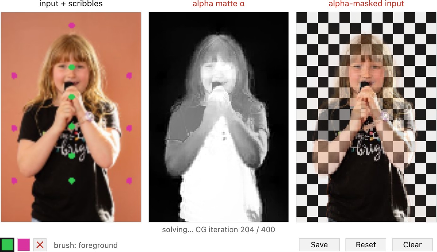
A line of robust / sampling hybrids (Wang and Cohen 2007 and the broader robust-matting literature) combined the two ideas (sample candidate $(F,B)$ colors per pixel like Bayesian matting, and impose the affinity smoothness of the matting Laplacian) and were the workhorse just before learning took over.

19.4.3 Deep-learning matting🔗⧉

The deep-learning era keeps the skeleton of the problem unchanged (still recover $\alpha$ from the matting equation) and swaps the hand-built prior (the color model, the color-line affinity) for a function fit to data (a recurrence of L7.6show: a learned operator in place of a hand-designed one). What it buys is the ability to learn the appearance of hair, fur, and motion blur from examples rather than assuming a local color line; what it costs is everything that comes with data dependence, and, as we will see, the data is the binding constraint.

Deep Image Matting predicts alpha from an image and trimap, with a refinement network and alpha/compositing losses (Xu et al. 2017). Its Composition-1k test set contains 1,000 synthetic composites from 50 test foregrounds; the training set is separate. Splitting by foreground identity matters because different backgrounds around the same object are not independent held-out subjects.

Trimap-free portrait methods such as MODNet predict alpha from one image under learned subject and capture assumptions (Ke et al. 2022 (MODNet)). Background matting uses an additional empty-scene photograph (Sengupta et al. 2020 (Background Matting); Lin et al. 2021). A clean plate supplies extra evidence but requires registration and consistent background appearance. Check each model's actual inputs instead of treating all low-interaction methods as equivalent.

For video, evaluate boundaries while they move and through occlusion. A fast single-frame model is not automatically temporally coherent, and a temporal objective can trade flicker for lag or persistent errors. Background-matting methods also depend on registration and the validity of the clean plate. Synthetic training composites provide useful alpha labels but may omit spill, interreflection, camera processing and capture blur found in real scenes.

Synthetic compositing makes a training example by placing an extracted foreground, with its known matte, over another background. This reuses an expensive annotation many times. It also leaves the foreground illuminated by its original surroundings: the new background does not automatically cast light onto it or appear in its reflections. That is a concrete reason why additional synthetic examples need not remove the gap to a real photograph. For video, the historical alternative is rotoscoping, with an artist tracing and correcting moving boundaries across frames. Temporal models automate part of that work, but ambiguous edges still require inspection.

19.4.4 Generative matting🔗⧉

The newest wave brings foundation models and generative priors to bear. They help, but the hard cases remain.

Segment Anything (SAM) (Kirillov et al. 2023) is the entry point, a promptable segmentation model trained on a billion masks: click a point, drag a box, or ask for "everything," and it returns clean masks for arbitrary objects with no per-class training. SAM collapses GrabCut's whole interaction (rectangle, color model, iterate) into a single prompt against a huge pretrained network, and it is the "cut anything" front-end that now feeds masks and trimaps to everything downstream. But SAM produces binary masks; it solves segmentation, not matting, and on its own gives you back the hard-edged hair problem.

A segmentation mask can be converted into a trimap and refined by a matting network, as in Matte Anything (Yao et al. 2024 (Matte Anything)). Preserve an uncertainty band around possible mask errors. Diffusion matting is another inference design; it does not automatically imply a text-to-image foundation model trained on billions of photographs. DiffMatte specifically develops iterative alpha estimation with a lightweight diffusion decoder (Diffusion for Natural Image Matting).

Inspect the predicted alpha and foreground color separately. Compositing error alone may hide compensating mistakes in those quantities. Evaluate on contrasting new backgrounds, fine edges and real captured examples; for video include flicker, lag and changing visibility. A plausible boundary is not evidence that its opacity was measured accurately.