38.3 Motion and video magnification⧉
The human visual system has limited spatio-temporal sensitivity, but many signals that fall below that threshold are perfectly real and perfectly informative. Human skin reddens slightly with each heartbeat as blood pulses through the capillaries, a color change usually too faint for the eye to register, yet it carries your pulse rate. A tall building sways a few millimeters in the wind; a crane, a bridge, a guitar string each tremble at frequencies and amplitudes the eye smooths away. A sleeping infant's chest rises by a hair with every breath. None of this is invisible because the light is missing. A camera can record these changes as small variations in pixel values, provided its exposure, frame rate, noise level, and compression preserve them. It is invisible because the changes are small and we are not built to see small. The goal of this chapter is to amplify subtle temporal variation in ordinary video: take a video and amplify the variations the eye misses until they are plain to see, turning the camera into an instrument that reveals motion and color change otherwise beyond human perception.
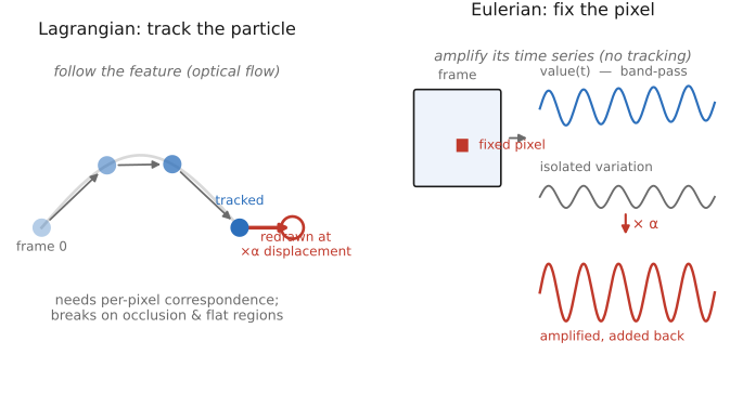
The chapter uses a distinction from fluid dynamics: Eulerian versus Lagrangian. There are two ways to watch a moving fluid. The Lagrangian view rides along with a particle: you pick a parcel of water and follow it as it travels, asking where it goes. The Eulerian view stands still: you fix a point in space and watch what flows through it, asking how the velocity at that location changes over time. The same fork confronts anyone who wants to amplify motion in video. The Lagrangian approach tracks features as they move from frame to frame (compute the Chapter 12.8, Optical flow), then redraw each feature at an exaggerated displacement. It works, and it was the first approach Liu et al. 2005, but it inherits all the difficulty of tracking: occlusions, featureless regions, and the brittleness of estimating motion at every pixel. The Eulerian approach refuses to track at all. Sit at a fixed pixel, treat its value over time as a one-dimensional signal, and amplify the temporal variations in that signal. It needs no correspondence, no flow, and no warping, spatial decomposition followed by temporal signal processing at fixed image locations. That choice is what makes Eulerian video magnification simple, fast, and the centerpiece of this chapter.
When the change you want to amplify is small, do not track it. Fix your viewpoint and process the time series at each pixel. Tracking (Lagrangian) is general but brittle: it needs correspondence, which fails on occlusion and texture-less regions. Amplifying-in-place (Eulerian) trades that generality for robustness and speed, and for small motions the trade is favorable: a linear, per-pixel pipeline that parallelizes easily and needs no motion estimation at all. The cost is that the approximation is only valid for small amplitudes and limited amplification; push it too far and it breaks (next sections). Choose the Eulerian frame whenever the signal is subtle and the budget is tight.
38.3.1 The Lagrangian precursor: track, then exaggerate⧉
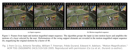
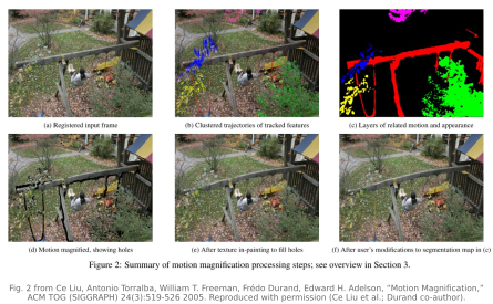
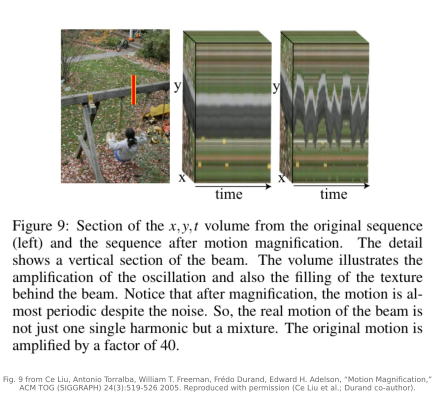
The obvious approach came first. Motion Magnification Liu, Torralba, Freeman, Durand and Adelson 2005 is the Lagrangian route in full: run Chapter 12.8, Optical flow to recover each feature's tiny displacement $\delta(t)$, cluster the trajectories into coherent layers, scale the displacement $\delta(t)\to(1+\alpha)\,\delta(t)$, and warp the frame to re-render the exaggerated movement. It is physically explicit and intuitive. You measure how far each thing moved and draw it moving farther. It is also fragile: it inherits every failure mode of optical flow, including occlusion, the aperture problem, and sub-pixel error, and estimating tiny motions accurately is precisely the regime where flow is weakest. It is general in principle but brittle in practice, and it cannot touch a pure color change (a pulse) because there is no point to follow. This is the method the Eulerian frame was invented to escape.
38.3.2 Eulerian video magnification: amplify the time series at each pixel⧉
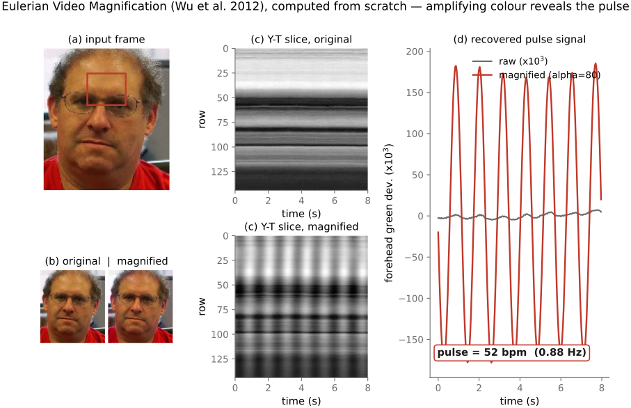
Start with the easiest version, amplifying a color change, because there the Eulerian recipe is almost too simple to believe. Point a camera at someone's face, hold it steady, and consider a single pixel on their cheek. Plot its value over time and you get a nearly-flat line with a tiny ripple: the ambient color, plus a minuscule periodic reddening synchronized to the heartbeat. The pulse is in that ripple, maybe a fraction of a percent of the signal, utterly swamped. To reveal it:
- Pick the band you care about. A pulse at 60 beats per minute is a 1 Hz signal. Choose a band that covers the rates expected in this recording, rather than imposing one narrow band on every person. Build a temporal bandpass filter tuned to that range and run it along each pixel's time series. The filter passes the heartbeat ripple and rejects out-of-band drift and noise; lighting variation, motion, and noise within the selected band remain. This is ordinary one-dimensional signal processing, the Chapter 6.3, Fourier-domain habit of isolating a frequency band, applied along the time axis instead of space.
- Amplify it. Multiply the band-passed signal by a factor $\alpha$, say $\alpha = 100$, and add it back to the original. The pixel's mean color is unchanged; only its tiny periodic excursion is now $1+\alpha=101$ times its original amplitude for an ideal unit-gain passband.
- Reconstruct. Do this at every pixel and play the video back. The face now visibly flushes and pales in time with the pulse. A signal that was below perception is now unmistakable, and you can read the heart rate straight off the screen (peak-detect the amplified trace and count).
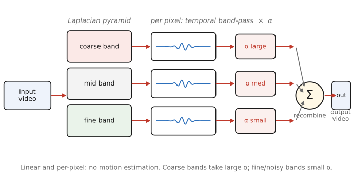
That is the entire algorithm for color magnification: per-pixel temporal bandpass, scale, add back. There is one practical refinement. The pulse signal is spatially smooth (a whole region of cheek reddens together) while the noise is spatially fine, so we first spatially blur or downsample the frame, pooling pixels into a coarse pyramid level, before temporal filtering. Averaging over a neighborhood raises the signal-to-noise ratio (the √N averaging of Chapter 13.2, Denoising by averaging) while sacrificing spatial detail; this is useful when the desired color change is spatially smooth. This is where the linear pyramid of Chapter 6.6, Pyramids and wavelets enters: decompose each frame into spatial-frequency bands, temporally filter and amplify each band, and collapse the pyramid back. Coarse bands carry the clean low-frequency signal; we can amplify them hard and the fine, noisy bands gently or not at all (Figure 38.3.5).
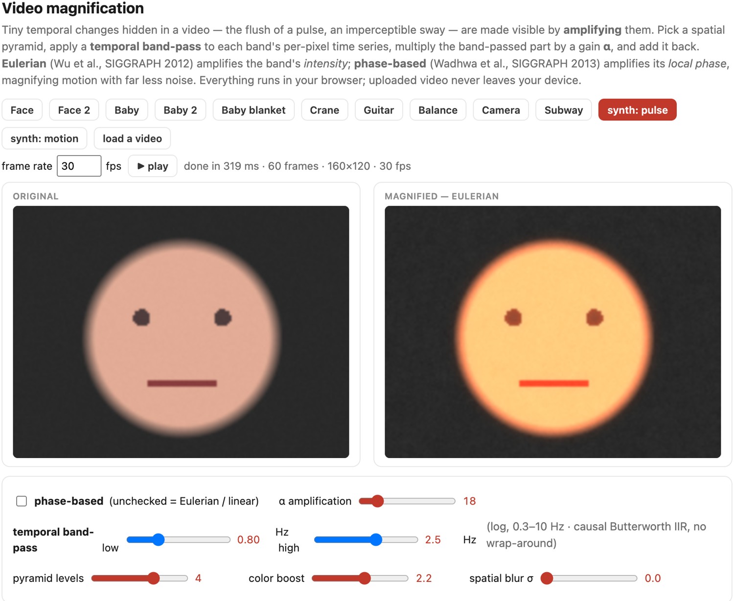
How do you band-pass a pixel's time series in practice? The textbook route is the ideal (brick-wall) Fourier filter: take the whole clip's time series, FFT it, zero every bin outside the band, invert. It is exact and one line of code, but it has two flaws for video. It is not causal: it needs the entire clip in memory at once, so it cannot run live as frames arrive. And the FFT treats the signal as periodic, so the end of the clip wraps around onto the beginning, the same circular-convolution wrap-around as spatial FFT filtering, and that seam leaks as ringing and ghosting at the temporal boundaries. The practical choice is a recursive (IIR) filter, and the classic is the Butterworth. A Butterworth filter is the maximally flat one: its passband is as flat as possible (no ripple), rolling off smoothly rather than as a brick wall. You build a band-pass as the difference of two Butterworth low-passes, one at each cutoff frequency, and each low-pass is a tiny recurrence. Every output sample is a fixed weighted combination of the last few input and output samples. Because it feeds its own output back (that is the "infinite impulse response"), it needs only a handful of stored values: O(1) memory, causal, real-time, and with no notion of the signal being periodic there is no wrap-around. The price is a gentler roll-off and a phase delay. Both are minor here, and the phase can be canceled by running the recurrence forward then backward. This is what the interactive demo below uses: a causal second-order Butterworth band-pass, per pixel, per pyramid band.
38.3.3 Why amplifying brightness amplifies motion⧉
Color magnification is intuitive because we directly scale the color change. The same operation, amplifying a brightness variation in place, also amplifies motion, even though we never tracked anything or moved a single pixel. It rests on the same first-order link between intensity and motion that underlies Chapter 12.8, Optical flow.
Here is the principle, in one dimension. Consider an edge, an intensity profile $I(x)$ that ramps from dark to light, and suppose between two frames the whole profile shifts by a tiny amount $\delta$. The new frame is $I(x - \delta)$. For a small shift, the first-order Taylor expansion says
Read it in words: a small spatial motion $\delta$ shows up, at a fixed location $x$, as a small temporal change in brightness equal to $-\delta$ times the local image gradient. The motion and the brightness wiggle are the same thing to first order, which is exactly the brightness-constancy relation of optical flow. Now do the Eulerian move: take that temporal brightness change $-\delta\,\partial I/\partial x$, multiply it by $\alpha$, and add it to the already shifted frame. The reconstructed signal becomes
The amplified frame looks just like the original profile shifted by $(1+\alpha)\,\delta$, so the motion has been magnified by the factor $(1+\alpha)$, without our ever estimating $\delta$ or warping anything. We amplified a brightness ripple at a fixed pixel and got an exaggerated motion for free, because for small displacements the two are linearly interchangeable. This is why the Eulerian method works: it converts the hard geometric problem of motion amplification into the easy signal problem of brightness amplification (Figure 38.3.6).
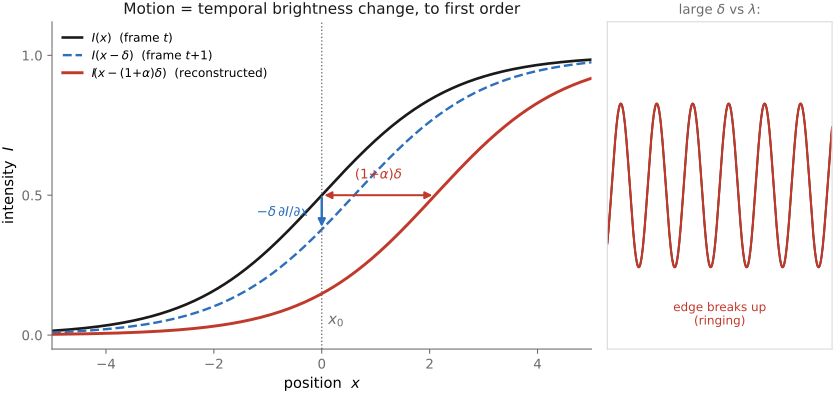
The same derivation tells us where it breaks, and we should not gloss over it (this is the method's central limitation). The Taylor expansion is only good while the displacement $\delta$ is small compared to the spatial wavelength $\lambda$ of the image structure, small compared to how fast the brightness varies in space. Amplify too hard, or apply the method to a motion that is already not-so-small, and $(1+\alpha)\,\delta$ outruns the linear regime: the added term no longer equals a clean shift, and the edge breaks up into ringing, halos, and amplified noise rather than moving cleanly. There is therefore a limit: the usable amplification $\alpha$ depends on the spatial wavelength $\lambda$, beyond which the intensity-based method degrades. Sharp, high-frequency structure (small $\lambda$) tolerates the least amplification; smooth, blurry structure (large $\lambda$) the most. The fix for this limit is the next section's subject.
38.3.4 Phase-based magnification: move the motion into phase⧉
The intensity method amplifies $\delta\,\partial I/\partial x$, a quantity that mixes the motion $\delta$ with the image's own contrast $\partial I/\partial x$, so noise (which also has a gradient) gets amplified alongside signal, and the small-displacement assumption is tight. Phase-based video motion processing Wadhwa et al. 2013 reduces these problems by changing what we amplify. The key fact comes from the same place as the Fourier shift theorem: when a signal translates, the amplitude of its frequency components is unchanged and the entire motion is carried in their phase. Shift a sinusoid and you don't change how big it is, only where its peaks fall, which is its phase. So instead of amplifying a brightness difference, measure the local phase and amplify the phase variation over time.
Concretely, decompose each frame with a complex steerable pyramid, a Chapter 6.6, Pyramids and wavelets whose sub-bands are localized in space, scale, and orientation and come with a local phase at every pixel (like a local Fourier transform). A small local motion shows up as a small change in that local phase over time. Now run the Eulerian recipe on the phase signal: band-pass the temporal phase variation, multiply by $\alpha$, and resynthesize the pyramid with the phases shifted. For a locally sinusoidal component, phase shift represents translation. Adding $\alpha$ times the filtered phase variation gives a total factor of $1+\alpha$ for motion in the passband. Phase wrapping, low-amplitude bands, occlusions, and motion beyond the spatial support still limit this approximation.
This buys two real improvements. First, less noise: the method keeps sub-band amplitudes unchanged instead of multiplying their fluctuations. Phase estimates are still noisy when contrast is weak, so amplitude-weighted smoothing and reliable-band selection matter. Second, larger amplifications before breakup: working in phase respects the structure of translation better than the first-order intensity approximation, so you can push $\alpha$ much higher before edges fall apart. The cost is more computation: a complex, oriented, multi-scale pyramid instead of a plain Laplacian one, but the quality gain is large enough that phase-based processing is the method of choice when the budget allows. (A faster, real-time variant uses a Riesz-pyramid approximation of the same idea Wadhwa et al. 2014.)
38.3.5 What it reveals: vital signs, structures, materials, modes⧉
With a near-free microscope for temporal change, the applications fall out by choosing which temporal band to amplify and where to point the camera.
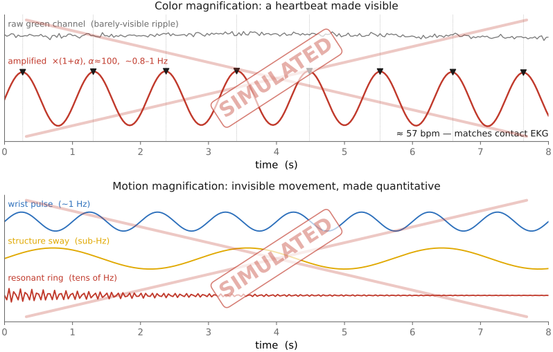
Vital signs, contactlessly. Tuned to an appropriate band, color magnification can reveal pulse-related changes in facial video without an electrode touching the skin. Demonstrations have compared recovered rates with contact measurements; agreement depends on motion, lighting, skin visibility, and camera quality. This is the basis of remote photoplethysmography Poh et al. 2010 (rPPG), recovering vital signs from an ordinary webcam. Tuned to the breathing band it reads respiration. This is medicine's interest in the method: monitoring the fragile (premature infants, burn patients) where contact sensors are awkward or harmful.
Structural and material analysis. Point the camera at a building, a crane, or a bridge and amplify the sub-hertz band, and the structure's gentle sway under wind and traffic becomes visible. This gives a non-contact way to watch how a structure deflects and where it is stiff or slack. Amplify a guitar's body or a wine glass and you can see it ring. Quantitative displacement measurement also needs image-scale calibration and a valid motion model; knowing the display amplification $\alpha$ alone does not give displacement in millimeters.
Vibration modes. Drive an object at its resonant frequencies and different parts move in characteristic patterns, the modal shapes illustrated by Chladni plates (sand on a vibrating plate collecting at the still nodal lines) and with laser interferometry. Motion magnification reveals these modes passively, from ordinary video, by amplifying each resonant temporal band in turn and watching which regions of the object move together and which stay nodal. This is the bridge to the next chapter: an object's tiny, mode-shaped vibrations, made visible here, also carry sound, and recovering that sound from the same kind of micro-motion is the visual microphone.
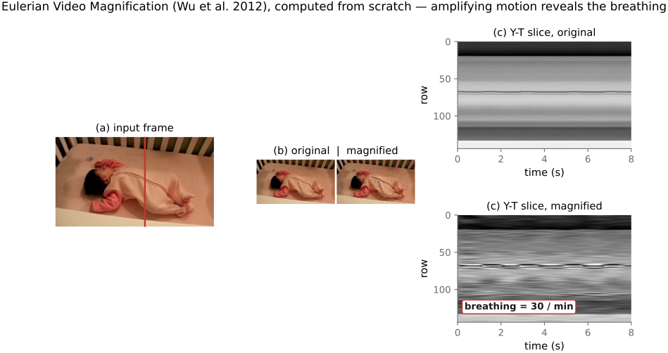
By refusing to track and instead doing per-pixel signal processing, motion magnification trades generality for a method that is linear, fast, and robust in exactly the regime that matters, small and subtle change, at the price of a small-amplitude approximation that phase-based processing then loosens. It is a near-perfect instance of the book's measure-then-process stance: when the camera preserves enough of the small temporal signal, processing can make it visible. The next chapter takes the same instrument and listens to it.
Recap: big lessons of this chapter
When the change you want to amplify is small, do not track it. Fix your viewpoint and process the time series at each pixel. Tracking (Lagrangian) is general but brittle: it needs correspondence, which fails on occlusion and texture-less regions. Amplifying-in-place (Eulerian) trades that generality for robustness and speed, and for small motions the trade is favorable: a linear, per-pixel pipeline that parallelizes easily and needs no motion estimation at all. The cost is that the approximation is only valid for small amplitudes and limited amplification; push it too far and it breaks (next sections). Choose the Eulerian frame whenever the signal is subtle and the budget is tight.