24.5 Colorization⧉
Hand a computer a black-and-white photograph (a 1930s street scene, a frame of silent film, an ancestor's portrait) and ask it to color it. The result can be striking: the past in color, as if it had been shot in color. It is also a textbook ill-posed inverse problem, and a uniquely instructive one, because it makes the part's recurring theme especially clear. In super-resolution and deblurring, how much the prior contributes depends on how much information the measurement lost. Colorization makes the ambiguity especially visible: a grayscale measurement preserves many spatial structures but collapses several color dimensions into one. That scalar constrains the possible colors, yet usually cannot tell whether a dress was red or blue. A prior or external reference must supply the missing distinctions. Colorization is the part's clearest proof that the prior is not a tie-breaker but the source of the signal.
24.5.1 One channel in, three channels out⧉
A common formulation uses $L^*a^*b^*$: retain lightness $L^*$ and predict chromatic coordinates $(a^*,b^*)$ (Chapter 4.1, Color space 101). YUV-like formulations instead separate a luma coordinate from two chroma coordinates. These are not interchangeable with physical luminance, and a historical grayscale photograph need not measure any of them exactly: film sensitivity, filters, and development affect its response. The synthetic training problem often starts with a known conversion from color to grayscale. That is two unknowns per pixel recovered from one measurement, under-determined by construction, exactly the shape of every recovery in this part, and the reason the answer needs a prior at all (L7.8, Chapter 14.1, What can super-resolution actually do?).
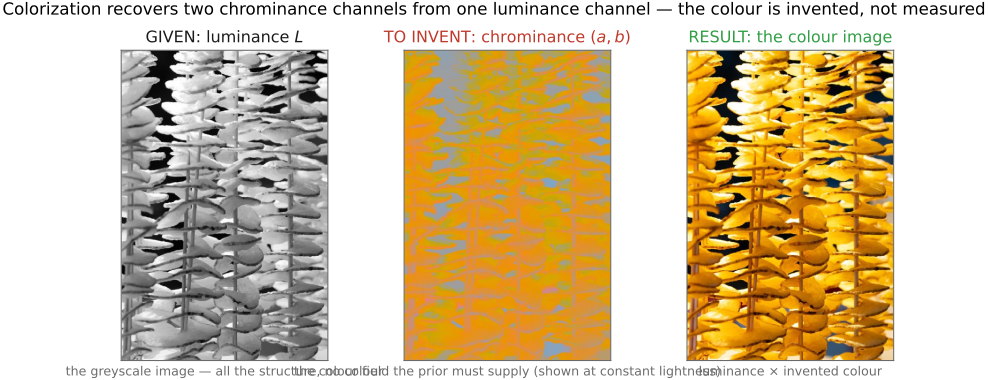
What makes it especially under-determined is that the missing quantity is multimodal. A gray car could plausibly be red, blue, silver, or black; a gray wall could be any pastel. The luminance does not merely under-specify the color: it leaves several genuinely different colors equally consistent. That fact drives the rest of the chapter, because the methods differ mostly in how they choose among the modes, and the automatic methods can fail precisely by refusing to choose.
What rescues the problem is that color is not free to vary pixel by pixel. A useful heuristic is that chrominance varies slowly within many regions and often changes at lightness boundaries. It is not a law: two different colors can have equal lightness, and a shadow can introduce a lightness edge without changing the material. And the world supplies strong statistical priors: skies and water trend blue, foliage green, skin to a narrow band of warm tones. Every method below is a different way of injecting one or both of these: local smoothness keyed to luminance edges, and global knowledge of what the world's colors usually are.
24.5.2 A spectrum of priors: scribbles, references, and learned models⧉
The methods sort cleanly by who supplies the color prior, from a human in the loop to a model trained on a large image collection (Figure 24.5.2).
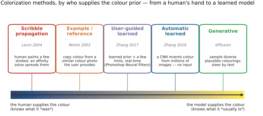
Interactive: the human picks the colors, the algorithm spreads them. The user crayons a few coarse color strokes and an optimization propagates them along luminance affinity (color flooding regions of smooth lightness and halting at luminance edges) so the human supplies which colors go roughly where and the algorithm supplies the spread. This is Levin, Lischinski & Weiss's (2004) scribble colorization, developed in full as the canonical filtering-becomes-optimization example in Chapter 10.3, Edge-preserving optimization — colorization (whose affinity construction is related to, but not identical to, the matting Laplacian in Compositing, segmentation and matting); here we only need that it sits at the human-supplies-the-prior end of the spectrum, accurate and controllable, but work, since every photograph needs someone who knows what color things were.
Example-based: a reference photo supplies the colors. Drop the scribbles and instead hand the system a color image of a similar scene: another beach, another face, another bowl of fruit. For each grayscale pixel, find the location in the reference whose neighborhood looks most alike (matched on luminance and a little local texture) and copy that location's chrominance across (Welsh, Ashikhmin & Mueller, 2002; refined to match within segmented regions by Irony et al., 2005). The prior is now "this other photograph," and the method is a color cousin of the histogram and color transfer of Chapter 8.7, Histograms and of the patch-copying in Chapter 21.1, Inpainting, texture synthesis: transport color from where it exists to where it is missing. It removes the per-stroke labor but trades it for the labor of finding a good reference, and it fails when no region of the reference matches a region of the target.
Fully automatic: a network supplies colors learned from examples. Train a convolutional network on a vast corpus of color photographs by the cheapest supervision imaginable: strip each one to grayscale, ask the network to predict its color, and compare against the original you hid (Zhang, Isola & Efros, 2016; Iizuka et al., 2016; Larsson et al., 2016). No human, no reference; the prior is the statistics of millions of images, learned (L7.6, Chapter 7.3, Deep learning). The network discovers the world's regularities (grass is green, lips are red, skies grade blue to white) and applies them automatically. This is the version that colors a museum's archive overnight, and it is where the multimodality of the problem turns from a footnote into the central design decision.
24.5.3 The multimodality trap: why naïve colorization goes muddy⧉
The key issue is multimodality, a lesson that reaches far past colorization. Suppose you train the automatic network the obvious way: predict the chrominance $(a,b)$ at each pixel and minimize the squared error against the true color, a regression loss. Ambiguous regions often become desaturated or muddy. The cause is not a weak network or too little data; it is the loss, and the multimodality we flagged at the start.
When a gray pixel could plausibly be red or blue, the squared-error loss is minimized not by guessing one but by predicting the average of the two, which lies between them in the chosen color coordinates. Red and blue need not average to gray; the relevant problem is that their average may be an unlikely color for this object. A network trained to minimize mean-squared error learns to output the mean of the conditional color distribution, and the mean of several plausible alternatives can have low probability under that same distribution. Averaging a multimodal distribution lands between plausible colors (Figure 24.5.4). The very ambiguity that makes colorization interesting is what a regression loss handles worst.
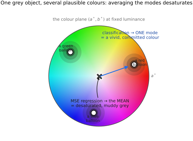
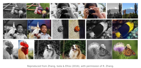
The fix is to stop averaging. Zhang and colleagues recast colorization as classification: quantize the $(a,b)$ plane into a few hundred color bins and have the network predict a probability over bins for each pixel, then pick (or take the expectation with a low "temperature" so it commits to a peak). Because real photographs are dominated by dull backgrounds, they also re-weight the rare, saturated colors up during training, so the network is not lulled into always betting on gray. The result is the saturated, decisive coloring of the gallery above. The deeper point generalizes: when plausible alternatives matter, model their distribution rather than relying only on its mean. The mean remains the optimal estimate for squared error, but that objective can conflict with plausible appearance. That is exactly why the generative chapter's diffusion models sample instead of average (L7.7, Chapter 7.4, Generative AI and diffusion): the muddy-brown colorization is the same failure as the blurry mean image, and "predict a distribution, then draw from it" is the same cure.
24.5.4 Closing the loop: learned priors with a human's hints⧉
The spectrum is not really a line with the human at one end and the machine at the other: its two halves combine in interactive learned colorizers. Real-time user-guided colorization (Zhang, Zhu, Isola et al., 2017) feeds the network the grayscale image and a handful of user color points, and is trained to honor the hints while filling everything else from its learned prior. It is the scribble idea of Levin with the hand-built affinity propagation swapped out for a trained model that already knows how the world's colors usually spread: drop one red dot on a balloon and the whole balloon turns a plausible red at once, because the network supplies the propagation and the prior the old optimization had to be told. This resolves the chapter's main tradeoff: the human chooses which colors where ambiguity matters, the learned model handles how they spread and everything left unspecified, and it runs at interactive speed. This division of labor is useful when a historical reference fixes a few important colors but leaves the rest uncertain. A hint should be checked in the result: learned propagation can spill across an object boundary or fail to honor the intended region. Automatic colorization has also become an ordinary menu item: Photoshop's Neural Filters, introduced in 2020, include a Colorize filter that proposes colors for a grayscale photograph and lets the user adjust them with focus points, the same automatic-then-hinted arrangement. Adobe does not document its model, so it illustrates the workflow rather than a particular method.
Generative colorization exposes several plausible answers. Many feed-forward colorizers are used to return one result, but adversarial training does not make a model inherently deterministic. Conditional GANs can include noise or dropout; in pix2pix-style systems, obtaining substantial diversity from that input is itself a challenge (Isola et al., 2017, Chapter 7.3, Deep learning). Diffusion and autoregressive models can sample alternative colorings, and text or color hints can steer them L7.7. Sampling represents ambiguity; it does not identify which sample matches the historical scene.
24.5.5 Plausible is not correct⧉
Which forces the chapter's plain caveat, and it is a sharp one. A colorized historical photograph is a confident guess, not a recovery. The grayscale photograph did not record enough independent color measurements to determine the original colors. Documents, surviving objects, or other photographs may still constrain them. The network supplies colors favored by its training and decoding procedure for a scene of that shape, which is often convincing and occasionally completely wrong: a dress that was green rendered a plausible blue, a uniform's true regimental color invented. Colorization fabricates information that looks like measurement, which is why it sits uneasily next to provenance and authenticity (Part 41, Image Forensics and Authentication): the output is indistinguishable, to the eye, from a real color photograph, yet inferred colors should not be presented as directly measured by the original photograph. Record which colors come from external evidence and which are guesses. Keep it distinct from false color: the deliberate mapping of non-visible data (infrared, depth, an electron micrograph's intensities) to hues, which makes no claim to be the scene's true color and says so plainly.
The same fact reshapes how you evaluate colorization. Measuring color error against the original photograph (a PSNR to ground truth) is misleading, because the original is just one of the plausible colorings, and a different-but-equally-plausible result is scored as a failure. One useful measure of perceptual plausibility is a colorization Turing test: show people the result and ask whether they believe it is a real color photograph. Zhang's automatic colorings fooled human judges roughly a third of the time, a measure of plausibility under that particular experiment, and a reminder that for every generative recovery in this part, "looks real" and "matches the held-out truth" are different questions, and the application determines which matters. Historical reconstruction also needs evidence-based fidelity; interactive editing needs control and consistency with user hints.
24.5.6 Where it sits⧉
Colorization is the limit case of the whole single-image part: the recovery in which the data supplies the skeleton and the prior supplies everything you actually came for. Read across the spectrum and you read the book's three reusable tools pointed at one task: solve an affinity-weighted optimization with a human's hints (Chapter 10.3, Edge-preserving optimization — colorization), transport color from an example (Chapter 8.7, Histograms, Chapter 21.1, Inpainting, texture synthesis), learn the prior from data (Chapter 7.3, Deep learning), and finally sample it (Chapter 7.4, Generative AI and diffusion). Related affinity constructions return in matting (Compositing, segmentation and matting); the same multimodality lesson returns as why diffusion samples; the same caveat (plausible is not true) returns wherever a learned prior fills in what the measurement left out. Color is the most visible thing a prior can invent, which is exactly what makes colorization the cleanest place to watch one work.
For all that progress, colorization remains, quietly, one of the field's big open problems. Even after the leap from affinity-weighted optimization to diffusion, automatic colorization that is at once faithful (the recovered colors are the true ones, not merely plausible ones) and controllable is unsolved in general: the ground truth simply is not in a grayscale input, many colorings are equally consistent with it, and the gap between "looks right" and "is right" never fully closes. It is the sharpest standing reminder of this part's central caveat: a prior fills in what the measurement threw away, and plausible is not true.