33.5 Code in time (phase, amplitude)🔗⧉

A car crosses the frame at speed, you press the shutter, and the license plate comes back as a useless gray ribbon. The reflex is to blame the exposure, too long, and to wish you had used a faster shutter. But a faster shutter buys sharpness with light: cut the exposure tenfold and you let in a tenth of the photons, and the plate is now sharp, dark, and buried in noise. This is the same bargain Chapter 33.1, Wavefront coding faced for depth of field, and Chapter 30.1, Motion blur, temporal sampling, and resampling stated as one knob: a long exposure blurs, a short one starves. Coded exposure (Raskar, Agrawal & Tumblin 2006) refuses the bargain by a move that sounds, again, backwards: keep the same acquisition window, but chop the shutter open and closed many times during the single exposure, in a carefully chosen pattern, and then recover a sharp plate in software. The trick is the cleanest temporal example of the part's central move: optics encode, computation decodes.

33.5.1 Why ordinary motion blur is (almost) unrecoverable🔗⧉

The natural place to start is with why you cannot simply deblur an ordinary motion-blurred photo, because it is exactly the obstacle the flutter shutter is built to remove. We saw in Chapter 30.1, Motion blur, temporal sampling, and resampling that a frame is an integral over the exposure window: while the shutter is open for time $\tau$, the sensor accumulates light along the whole path a moving feature traces. For a feature moving at constant image-plane velocity, that integral is a convolution by a 1-D box kernel $k$, a flat segment of length $\lVert\mathbf v\rVert\tau$ along the motion direction, normalized to unit area. Blur is convolution; convolution inverts by deconvolution; so why not just divide it back out?

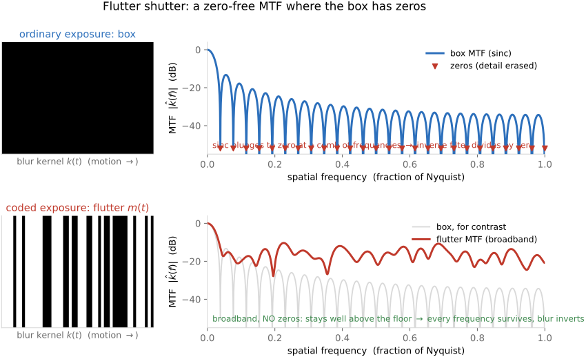
Because the box is a terrible kernel to invert. A box in space is a sinc in frequency, and a sinc crosses zero, periodically and infinitely often. At every one of those zeros the blur's frequency response is exactly nothing: the box has multiplied that spatial frequency by zero. As Chapter 16.4, Blind deblurring makes precise, a frequency the kernel killed is unrecoverable. Dividing by zero in the inverse filter recovers no signal, only amplified noise. The flat box does not merely scramble the moving object's high frequencies, it erases a comb of them, and stamps the gaps right where text and edges live. This is why deblurring an ordinary motion-blurred plate, even when you know the exact speed, comes back ringing and wrong: the information at the box's zeros was never recorded. Worse, if you do not know the speed (the usual case) you are also blind to which box to invert, the chicken-and-egg of Chapter 16.4, Blind deblurring.

33.5.2 The flutter shutter: chop the exposure into a code🔗⧉

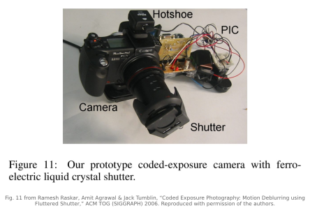
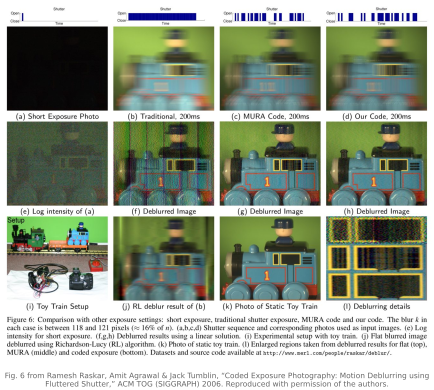
Here is the leap, and it is the temporal twin of the cubic phase plate. Instead of accepting the box that a continuously-open shutter hands you, the flutter shutter re-engineers the temporal window so that its frequency response has the one property deconvolution craves: a response bounded away from zero over the reconstruction band. During the same total acquisition window $\tau$, the shutter is snapped open and closed many times, following a fixed binary on/off pattern: a temporal code $m(t)$, a string of 1s and 0s. Raskar and colleagues use a pseudo-random sequence of around fifty-two chops chosen, by a short search, so that the resulting kernel's spectrum stays as flat and high as possible across the band. Physically the flutter is just a fast electronic gate in front of an ordinary camera: their prototype drives a ferro-electric liquid-crystal shutter with a small microcontroller, snapping it opaque and clear on the coded schedule during one otherwise-normal exposure.

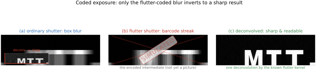
The effect on the blur is the whole point. A moving feature now deposits its light as a broken, barcode-like streak (bright where the shutter was open, dark where it was shut) rather than a flat ribbon, and the blur kernel $k$ is that barcode rather than a box (Figure 33.5.2⛶ fullscreen). The code is chosen so that $k$'s frequency response is broadband and zero-free: it stays well above zero everywhere across the band, so the targeted spatial frequencies are better preserved. Finite gate duration, optics, and sampling still limit the available band. The captured frame still looks blurred, and often more fragmented than an ordinary blur, but that ugly intermediate is the part introduction's "code that is not yet a picture." Once the motion is also known or estimated, the code determines a spatial blur kernel. Regularized deconvolution can recover detail that a box exposure would suppress much more strongly.

Note what the flutter does not do: it preserves the full acquisition window while reducing the time actually spent collecting light. The object is smeared over the full $\tau$, so motion blur is just as large: the flutter does not freeze the motion, it makes the blur decodable. And because the shutter is open for roughly half the total window, the method keeps about half the light of a full exposure, far more than the brief snapshot that would freeze the same motion. You pay one stop of light to convert an unrecoverable blur into an invertible one.

33.5.3 The decode: one deconvolution, a sharp moving object🔗⧉

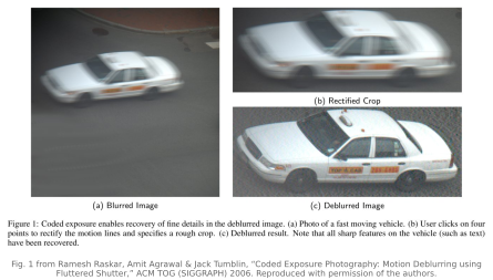
The pipeline is therefore exactly the encode→decode pair of the part introduction, run in time. The optics encode: the fluttering shutter spreads the moving object into a broken, broadband, information-preserving streak, an intermediate capture that is uniformly, decodably blurred and not yet a picture. The computation decodes: a single deconvolution by the known flutter kernel restores the object's sharpness, recovering the comb of frequencies an ordinary box would have killed. The result is a sharp moving subject from a normal-length exposure, with no flash, no high ISO, and no frozen-but-noisy snapshot (Figure 33.5.4⛶ fullscreen).

Two caveats keep the accounting straight. First, the flutter blur is still a blur the size of the full streak, so you must know (or estimate) the object's motion to pick the right kernel; coded exposure makes the blur invertible, it does not make it self-evident. Raskar and colleagues recover the streak length from the cutoff in the captured spectrum or from a user-marked extent, then deconvolve. Second, as always with deconvolution, sharpening costs noise: restoring the high frequencies amplifies whatever noise rode at them, so the recovered frame can carry substantial noise when the retained response is small. Avoiding zeros improves conditioning but does not guarantee a small noise penalty (contrast the catastrophe of inverting a box in Chapter 16.4, Blind deblurring). The trade is the usual coded-imaging bargain: accept a controlled, invertible degradation and a noise penalty in exchange for improved recovery of a moving subject from a long acquisition window.

33.5.4 Amplitude in time, and phase in time🔗⧉

Naming what the flutter shutter codes places it in the part's grid. The shutter does only one thing: it passes light or it blocks it, so the flutter is an amplitude code in time: a binary on/off modulation $m(t)\in\{0,1\}$. This is the exact temporal cousin of Chapter 33.3, Coded aperture, which puts a binary on/off amplitude mask in space across the pupil; one codes which directions contribute, the other codes which instants contribute. And like every amplitude code it is lossy: blocking the shutter half the time throws away half the light. That is the price of coding amplitude, in time as in space.

Coded illumination implements a temporal code by changing the emitted intensity rather than rejecting ambient photons at the shutter. Pulsing a strobe or shifting its timing still modulates intensity; it is not the optical-phase counterpart of a transparent phase plate. The phase of a periodic illumination waveform means its timing within a cycle. Phase-based time-of-flight systems measure the delay of that modulation using multiple demodulation channels or phase samples. Neither use implies that every photon is collected or that temporal coding is lossless.

33.5.5 Coded strobing, temporal multiplexing, and compressive video🔗⧉

Once you can code the time axis, the same intermediate-code logic buys more than deblurring. Three uses follow, each a temporal echo of something already in this part.

High-speed beyond the frame rate. Spatially varying coded shutters can mix sub-frame instants into one sensor read and reconstruct a short burst under a motion, sparsity, or learned prior. A single global strobe pattern does not independently label every instant in the integrated image: without additional measurements or assumptions, many videos produce the same sum. This is an underdetermined inverse problem, as in Chapter 33.2, Compressive sensing, and recovered motion outside the ordinary frame-rate band remains conditional on the model.

Separating illumination. Give each light source a temporal code and record enough independent exposures or demodulation channels to separate their contributions. The matrix of integrated code weights must have sufficient rank for the unknown source images. One ordinary integrated frame supplies only one weighted sum per pixel; assigning several source codes does not by itself make that sum separable. This is the temporal relative of illumination multiplexing and direct/global separation elsewhere in the book.

Compressive video. Generalize the per-pixel coded shutter and a single sensor frame becomes a coded projection of a whole short clip, many sub-frames collapsed onto one read, by a pixel-wise temporal code, from which the clip is reconstructed under a sparsity or learned prior. The encoder is a coded exposure pattern that varies per pixel; the decoder recovers the video. It is the purest statement that time is just another axis of the operator $A$ from Chapter 6.7, Image formation as a linear system, and that coding it is the same discipline as coding space.

33.5.6 Motion-invariant photography🔗⧉

The flutter shutter codes the blur to be invertible but leaves it speed-dependent: to deconvolve a frame you still have to know how fast the object moved, and different objects moving at different speeds carry different kernels. Motion-invariant photography (Levin, Sand, Cho, Durand & Freeman 2008 Levin et al. 2008 (motion-invariant)) makes a more aggressive move. It engineers an approximately common blur over a chosen range of one-dimensional object velocities, allowing one deconvolution without estimating each velocity separately.

The trick is to move the camera during the exposure, sliding the sensor (or panning) along a constant-acceleration, parabolic trajectory. The key reason it works is simple. An object moving at constant velocity traces a straight line in space–time; the camera's parabolic sweep means that over the exposure the camera's own velocity passes through every value in a range. For an object moving along that axis within the swept velocity range, there is an instant when the camera moves at exactly that speed, and at that instant the object is momentarily sharp, and the smear it accumulates the rest of the time has a shape that turns out to be independent of the object's velocity (to first order, for any speed in the swept range). Within this model, stationary and moving objects have approximately the same calibrated point-spread function (Figure 33.5.6⛶ fullscreen); this is the temporal sibling of the coded-aperture and wavefront-coding designs, and the linear-operator view of it is in Chapter 6.7, Image formation as a linear system.

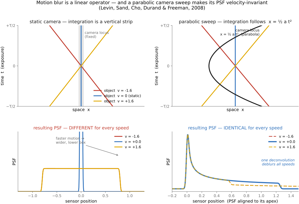
That invariance is the point. With one known, velocity-independent kernel, deblurring is a single non-blind deconvolution of the entire frame: no per-object motion estimation, no segmenting movers from background, none of the spatially-varying-blur misery that ordinary motion deblurring drowns in (Chapter 16.4, Blind deblurring). The cost is symmetric to the flutter shutter's. Motion invariance assumes motion along a known 1-D direction (the sweep axis), so it handles horizontal traffic well but not motion across the sweep; finite sweep boundaries, acceleration of the subject, occlusions, and motion across the sweep break the approximation; and the static background, which an ordinary photo would have rendered razor-sharp, is now blurred along with everything else and must be deconvolved too. Flutter codes the kernel to be invertible and pays by needing the speed; the parabolic sweep codes it to be invariant and pays by committing to a motion direction and blurring the still scene. They are the two temporal answers to the question wavefront coding answered for depth: how do you turn a blur you cannot control into a blur you can decode?

33.5.7 Where it sits🔗⧉

Coded exposure is one member of a family, and naming its siblings places it. Along one axis it is a temporal amplitude code, the time-domain partner of the spatial-amplitude Chapter 33.3, Coded aperture and the contrast to an ideally nonabsorbing Chapter 33.1, Wavefront coding plate. It applies the same principle of designing the measurement operator for reconstruction. Temporal intensity coding should not be confused with modulation of optical phase. Along the other axis it sits beside motion-invariant photography (above): flutter reshapes the kernel to be zero-free but speed-dependent; the parabolic sweep makes it speed-invariant.

That deconvolution (how you invert a known, well-conditioned blur), and what to do when the kernel is not known, is the subject of Chapter 16.4, Blind deblurring. Here we needed only the promise coded exposure relies on: a calibrated blur with adequate response over the reconstruction band can be inverted with regularization, within the limits imposed by noise and model error. Flutter the shutter in the right pattern and a fast subject stops being something you freeze with light and becomes something you compute.