14.2 Multi-frame super-resolution⧉
In a one-dimensional sampling example, a second capture shifted by half a pixel fills the gaps in the first grid. In two dimensions, doubling sampling density along both axes needs complementary offsets along both axes. Two frames do not generally supply a complete grid with twice the width and height.
Known shifts give additional equations for the same scene. Their rank and conditioning determine how much new information they provide. A practical reconstruction also uses assumptions about image smoothness, noise and motion; it is not free of priors.
The catch, in every real system, is that you do not know the shifts, you have to estimate them from the noisy aliased frames themselves, and the estimate has to be more accurate than the resolution gain you are trying to buy.
14.2.1 Sub-pixel shifts are extra samples⧉
Write the forward model per frame. Each capture applies its own displacement, then the same blur and downsampling as before:
Here $W_k$ maps the reference high-resolution image into frame $k$ before blur and sampling. For the same blur and full overlap, integer shifts on the coarse sensor grid repeat the sampling phase: they reduce independent noise but add no new spatial phases. Fractional shifts can add useful constraints, although clustered or collinear offsets may leave the system rank-deficient. A scalar $s$-fold enlargement in both dimensions needs at least $s^2$ full frames to match the number of unknowns without a prior; that count is necessary in this ideal model, not sufficient.
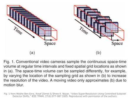
Natural hand motion can supply sampling diversity, but motion during each exposure also causes blur. A stationary tripod sequence repeats the sampling phase unless an actuator moves the sensor or optics. Pixel-shift cameras deliberately introduce offsets (Chapter 15.12, Hardware alternatives to the mosaic). A jitter camera explores controlled sampling over time (Ben-Ezra et al. 2005; Figure 14.2.1).
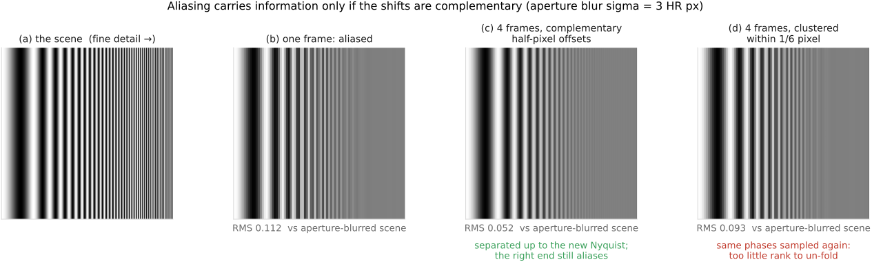
In the frequency domain, a translation multiplies each spectral component by a phase. Aliased components with different original frequencies acquire different phases across offsets, allowing a set of shifted frames to separate them when the resulting mixing system has sufficient rank (Figure 14.2.2). This is the frequency-domain construction of Tsai and Huang (Tsai & Huang 1984).
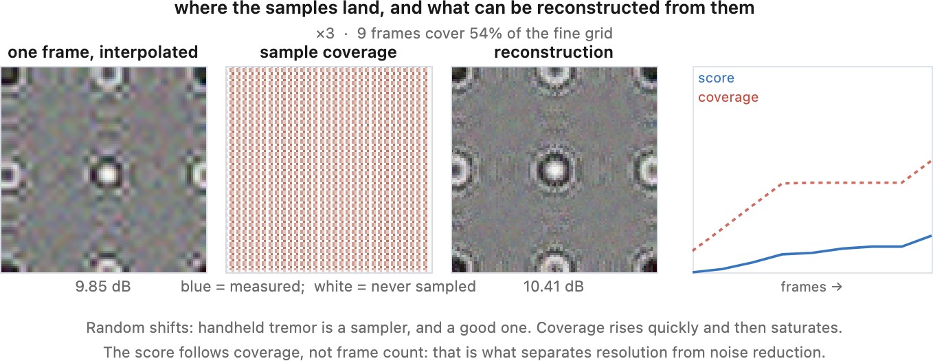
Offsets must provide well-conditioned sampling coverage, and the combined optical and pixel transfer must retain the desired detail. Noise, motion and calibration determine which weakly transmitted components are usable. There is no universal twofold gain that every burst reaches, nor a fixed frame count after which resolution cannot improve.
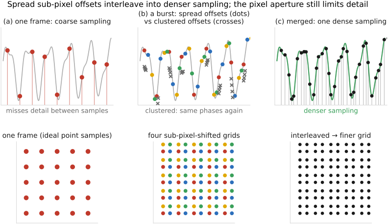
In one dimension, a second sample grid shifted by half a low-resolution pixel supplies positions between the first grid's positions. A second grid shifted by a whole pixel mostly repeats the same sampling phase over the overlap. The latter can still reduce noise and extend coverage, but it does not provide the same interleaving of fine-scale samples. Real pixels also integrate light over a footprint, so the half-pixel shift does not by itself guarantee recovery of frequencies suppressed by that integration or by optical blur. Controlled sensor shifts and measured hand motion are two ways to obtain sampling diversity; both require a reconstruction consistent with the actual footprints and scene motion.
Consider two frequencies that produce the same samples on one coarse grid. From that frame alone, their contributions cannot be distinguished. Translate the grid by a fraction of a pixel and the two frequencies acquire different phase changes because their original frequencies differ. The next frame therefore measures a different linear combination of the same unknown contributions. Enough suitably spaced observations can separate them, provided the optics transmitted them and the registration is accurate. This explains why aliasing in one frame can carry recoverable information in a burst: the additional measurements disambiguate a folding that a single measurement could not undo. Repeating exactly the same sampling positions improves noise but supplies no new phase combinations.
14.2.2 The classical formulations⧉
Tsai and Huang (Tsai & Huang 1984) formulated translated-frame reconstruction in the frequency domain. The derivation makes alias separation explicit under a common translational imaging model. Real blur, noise and finite boundaries require appropriate transfer functions and regularization.
Iterative back-projection (Irani & Peleg 1991) predicts the low-resolution frames from a high-resolution estimate and uses the prediction errors to update it. A least-squares implementation uses the adjoint of each complete forward operator, not an inverse geometric warp:
x = upsample(reference_frame, factor)
x_new = x
for it in range(maximum_iterations):
    gradient = zeros_like(x)
    for k in range(number_of_frames):
        residual = A[k](x) - frames[k]
        gradient += A_adjoint[k](residual)
    x_new = x - step * gradient
    if stopping_criterion(x_new, x):
        break
    x = x_new
return x_new
For $A_k=SBW_k$, this is gradient descent on $\tfrac12\sum_k\lVert A_kx-y_k\rVert^2$ when the adjoints are exact. A sufficient step bound is $0<\eta<2/L$, where $L=\lVert\sum_k A_k^{\mathsf T}A_k\rVert_2$. Sampling's transpose scatters residuals back to the sampled locations; a warp's transpose accumulates interpolation weights. Neither is generally ordinary upsampling followed by an inverse warp.
A prior adds a regularization step. Farsiu and colleagues (Farsiu et al. 2004) use an $L_1$ data term and regularization to reduce the influence of inconsistent samples. An outlier-resistant loss helps with some registration errors, but cannot make systematically wrong correspondences correct.
14.2.3 Registration is the hard part⧉
To gain a factor of two in resolution, the alignment has to be accurate to a small fraction of a pixel, better than the detail being recovered. Estimating that from frames that are aliased, noisy and low resolution is the central difficulty, and it has an unpleasant circularity: aliasing is what makes the extra information available, and aliasing is also what makes the frames disagree about where things are.
Three consequences show up in every system that works.
Coarse-to-fine alignment can reduce the influence of aliasing before refining the motion. Its coarse levels need enough structure and an appropriate capture range; it is a useful strategy rather than a requirement of every method.
Camera translation, depth variation and moving subjects can require local correspondence. Pure camera rotation is a case where a global homography may suffice. Choose the model for the scene and retain a measure of confidence.
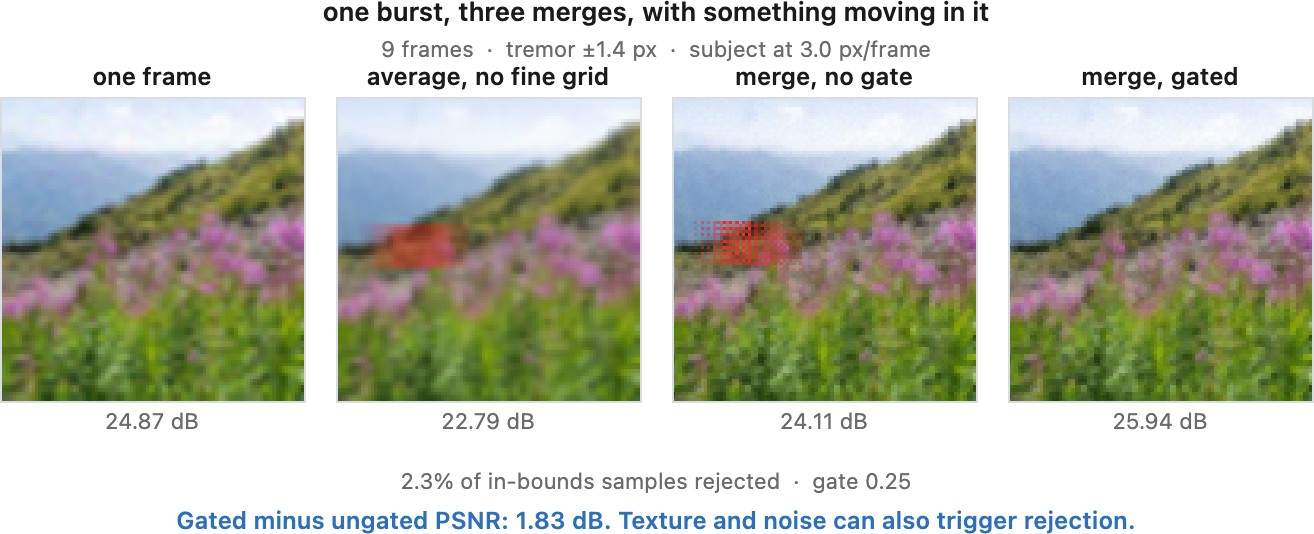
Where alignment fails, reduce the contribution of inconsistent frames or fall back to the reference. This sacrifices some resolution and noise reduction locally. A confidence mask is itself an estimate and can reject useful samples or accept wrong ones.
14.2.4 What actually ships⧉
This is the part of super-resolution that is deployed at enormous scale, and the deployed systems are worth reading as engineering.
Handheld multi-frame super-resolution (Wronski et al. 2019) is the clearest example. It runs on a phone, uses the hand's natural tremor as the source of sub-pixel shifts, and does something the classical formulation does not: it merges the raw Bayer frames directly onto a finer grid, so demosaicking and super-resolution happen in one step rather than in sequence. That is the same joint argument Part 15, Demosaicking and joint methods makes, and it wins for the same reason. The merge is a locally adaptive kernel regression whose kernels are steered by the local structure tensor, so the accumulation is anisotropic along edges, and a robustness model gates each frame's contribution per pixel.
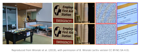
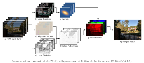
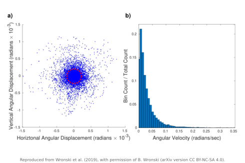
HDR+ (Hasinoff et al. 2016) and Night Sight (Liba et al. 2019) illustrate related burst machinery aimed at low-light quality. A product name does not identify whether a result uses one image, a burst, raw reconstruction or a generative prior; document the specific mode and version when evaluating a system.
The Wronski system combines raw reconstruction, alignment, adaptive interpolation and rejection of inconsistent samples. These stages explain its result more precisely than attributing every improvement to the output grid size.
Chapter 14.3, Learned burst methods describes learned alignment and fusion, and the paired captures used to train and test them.
Product examples also show why the labels can be confusing. Apple introduced Deep Fusion in 2019 as processing that combines multiple images using its neural engine (iPhone 11 announcement). Adobe's Enhance Details, introduced in 2019, improves raw demosaicking; its Super Resolution feature, introduced in 2021, enlarges a single photograph to twice the width and height and includes Enhance Details when applied to raw files (Adobe's technical introduction). These are concrete examples of different operations marketed around detail: multi-frame combination, improved color reconstruction, and learned enlargement. Their names do not tell us which extra measurements, if any, support the result.
14.2.5 The gain, and where it stops⧉
Noise reduction and sampling diversity provide different benefits. Repeated phases can still reduce independent noise; new well-spread phases can improve resolution when the transfer function permits it. The benefit of another frame depends on which constraints and which scene regions it adds. At fixed total exposure time, splitting capture into more frames also adds read-noise costs, as Chapter 13.2, Denoising by averaging derives.