36.5 Multi-view 3-D reconstruction: the classic pipeline⧉
Two views give depth; the opening chapter derived the algebra and deferred its estimation and the leap to many images. This chapter does both. With many views of a rigid scene, dozens of photos or the frames of a video, we can recover a consistent scene and camera configuration, ordinarily up to a global similarity transform: where every camera was, and a dense 3-D model of the scene. The catch is that the classical way to do it is a long pipeline of hand-built stages, each imperfect, with joint refinement needed to correct errors accumulated along the chain.
36.5.1 The pipeline, stage by stage⧉
The full chain reads: features → correspondences → fundamental/essential matrix + RANSAC → structure-from-motion (poses + sparse points) → bundle adjustment → dense multi-view stereo → mesh + texture (Figure 36.5.1). The first three stages are exactly the machinery built for automatic panoramas in Multiple exposure imaging (detect repeatable keypoints, describe them, match with the ratio test, reject outliers with RANSAC), reused here with the difference that now the camera translates between views, so depth does not cancel (unlike the homography case, where it did).
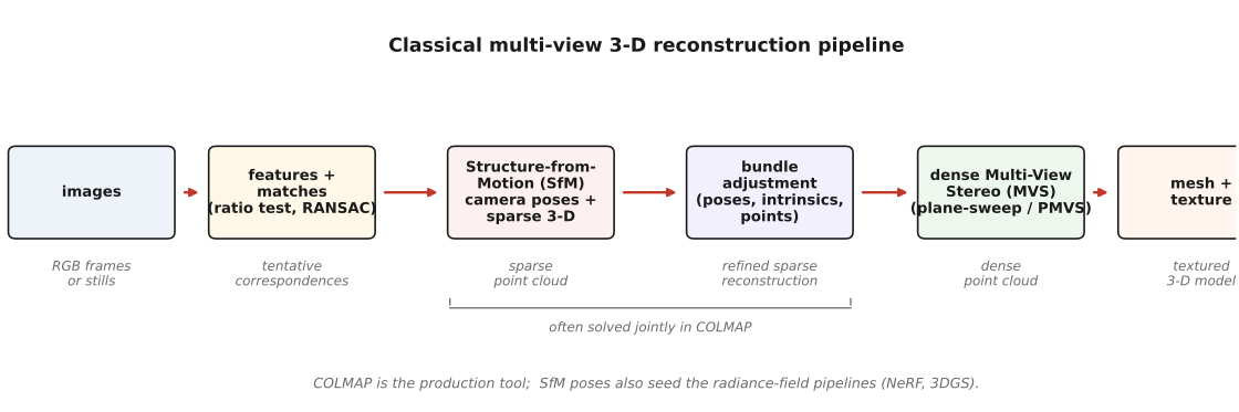
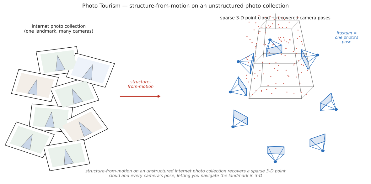
Structure from Motion (SfM) is the heart of the pose-recovery half. From sparse feature matches it estimates each camera's intrinsics (focal length, radial distortion) and extrinsics (rotation and translation), seeding them from the two-view essential matrix and incrementally adding cameras. The main refinement is bundle adjustment: a large non-linear least-squares optimization that jointly adjusts camera poses, selected intrinsics, and all 3-D point positions to minimize the total reprojection error: the pixel distance between each observed feature and where its 3-D point projects. As a free by-product, SfM hands you a sparse 3-D point cloud (the triangulated feature points). The production-grade open-source tool is COLMAP Schönberger & Frahm 2016, and the famous demonstration that this scales to the wild is Photo Tourism Snavely et al. 2006, which reconstructed landmarks like the Trevi Fountain and Notre-Dame from thousands of unstructured internet photos (different cameras, days, seasons, and crowds) and let a user fly between them.
The normalized eight-point algorithm supplies a useful concrete starting point for estimating $F$. Center and scale the image coordinates, form one linear equation $x'^{\mathsf T}Fx=0$ per match, and solve the homogeneous system by SVD. Reshape the solution into a matrix, set its smallest singular value to zero to enforce rank two, and undo coordinate normalization. Eight matches are the minimum for this linear estimator, not for every two-view solver. With known intrinsics, calibrated minimal solvers can use five matches. RANSAC tests hypotheses on held-out correspondences using a geometric or Sampson residual; the final estimate is refined on its inliers.
match features across candidate image pairs
for each pair:
    estimate two-view geometry robustly
    retain inlier correspondences and reject degenerate pairs
choose a well-conditioned seed pair
recover pose; triangulate points in front of both cameras
while an image has enough matches to existing 3D points:
    estimate its pose from 2D-to-3D correspondences
    triangulate new tracks; reject inconsistent observations
    jointly refine cameras and points by bundle adjustment
estimate dense depth in supported views; fuse consistent surfaces
Noisy viewing rays generally do not intersect exactly. Triangulation initializes a point by minimizing a ray or algebraic discrepancy, then can refine it by image reprojection error. Bundle adjustment extends that refinement to all observations:
Here $\mathcal O$ is the set of observed point-camera pairs, $u_{ij}$ a measured feature, $\pi$ the calibrated projection, and $\rho$ a robust loss. Fix a reference pose and scale to remove the similarity gauge; otherwise equivalent reconstructions leave the optimization underconstrained. Calibration parameters need not all be free, especially when the images provide weak evidence for them.
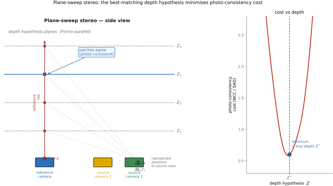
Dense multi-view stereo (MVS) then goes from the sparse cloud to a dense one. The workhorse idea is plane-sweep stereo: hypothesize a series of depths for each reference pixel, and for each hypothesis reproject the surrounding image patch into the neighboring views; the correct depth is the one where the reprojected patches agree, meaning they are photo-consistent across the views that see them (Figure 36.5.2). PMVS (Patch-based MVS) Furukawa & Ponce 2010 (PMVS) grows and filters small oriented patches, expanding from confident matches and discarding photo-inconsistent ones, scaling from ~100k seeds to tens of millions of surface points. (Modern learned variants such as cascade cost-volume MVS sharpen this further, but the photo-consistency principle is unchanged.)
Meshing and texture close the pipeline: fuse the dense point cloud into a continuous surface (a triangle mesh), then texture it from the input photos. To preserve the "shiny," view-dependent look of real specular surfaces, view-dependent texture mapping Debevec et al. 1996 (Façade) blends the actual input views per output viewpoint rather than baking one flat texture, an idea that anticipates the view-dependent color of radiance fields.
36.5.2 Why it is brittle: and why SfM survives anyway⧉
For all its power, the classic pipeline has well-known limitations, and they motivate everything that follows. It is slow, often taking minutes to days for a serious model. It assumes clean, opaque, roughly Lambertian surfaces, so it struggles on specular highlights (which move between views and break photo-consistency), on transparency, on fuzz like hair and foliage (no stable patches to match), and on textureless regions (no features to detect, no patches to compare, the same failure the stereo chapter flagged). It is a long chain, so errors at any stage accumulate. And it leaves holes wherever coverage or matching failed. These are exactly the pain points the radiance-field methods of Chapter 36.7, Photos → radiance fields and Gaussian splatting (NeRF, 3DGS) were built to fix: a differentiable appearance fit and representations that can model complex visibility and view-dependent appearance. They still face pose errors, inadequate coverage, and ambiguous geometry; fuzziness does not solve these automatically.
But the pipeline is not obsolete. Its first half, SfM for camera poses, is still the first step of most modern methods, NeRF and 3-D Gaussian splatting included: they run COLMAP to get the camera poses (and a sparse point cloud to initialize from) before they ever optimize a radiance field. The classic pipeline's pose machinery survives as a widely used front end, though some methods jointly estimate poses or predict them directly; it is mainly the dense reconstruction half that the new representations replace.