15.6 Learned demosaicking⧉
Fine fabric and thin diagonal structures can defeat local interpolation rules. A learned demosaicker uses a larger training collection to fit how sparse color samples map to full-color detail.
A synthetic training pair is easy to construct by selecting one component per pixel from a full-color image. Producing a representative clean target is harder: a processed photograph may already contain demosaicking, denoising, sharpening and compression artifacts, and its RGB channels need not be camera-linear responses.
Specify the color domain and how the target was prepared before treating remosaicking as a sensor simulation.
15.6.1 The data problem hiding inside a free training set⧉
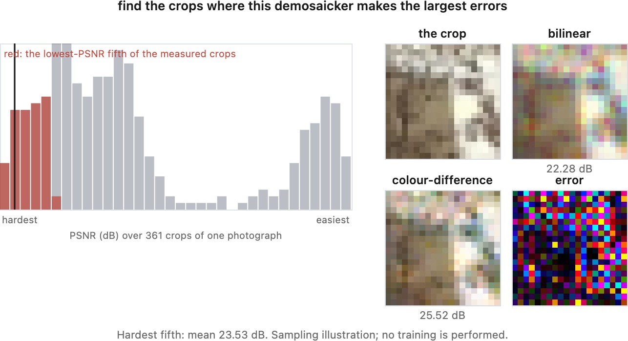
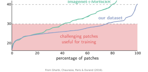
Uniformly sampled crops may underrepresent difficult patterns. If most loss comes from easy or common regions, training can leave rare artifacts insufficiently addressed. The actual error distribution should be measured.
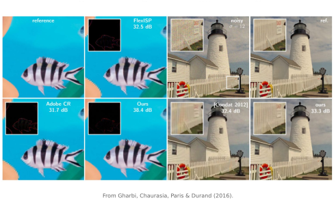
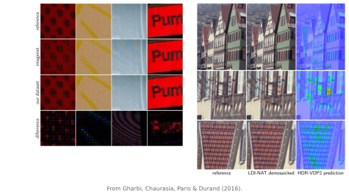
Gharbi and colleagues' contribution (Gharbi et al. 2016) was to notice this and to mine for the hard cases. Run a classical method over a large corpus, find the patches where it fails, and train mostly on those. The network then spends its capacity on moire, on fine diagonal structure, and on the color boundaries where the difference assumption breaks, which is where the remaining error actually is.
Hard-case mining changes what the network is trained to prioritize. Keep a representative held-out test set, and report performance on both ordinary and difficult scenes; otherwise a gain on mined cases can hide regressions elsewhere.
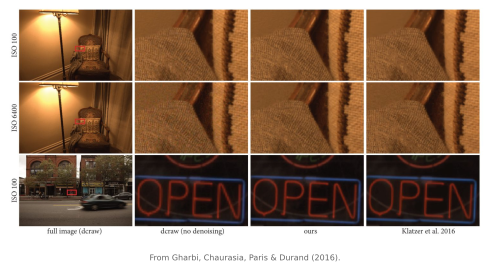
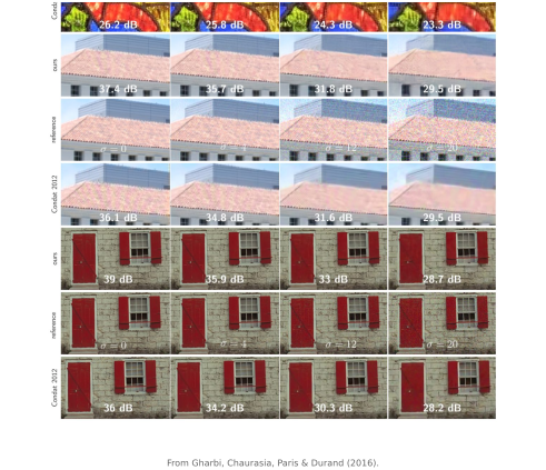
24 classic lossless images, the long-standing demosaick/denoise benchmark. <https://r0k.us/graphics/kodak/>. See the Chapter 45.16, Datasets appendix.
15.6.2 Architectures, briefly⧉
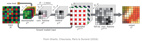
Gharbi et al. used a convolutional architecture and curated difficult examples (Gharbi et al. 2016). Later designs include explicit cross-channel guidance (Liu et al. 2020 (self guidance)), transformer/attention blocks (Xing & Egiazarian 2022 (RSTCANet)) and joint reconstruction tasks (Xing & Egiazarian 2021 (joint demosaic-denoise-SR)). Their differences matter only alongside the training data, loss, noise conditions and computation budget.
Two representation choices are particularly useful in implementing these models.
Pack the mosaic. Rearrange a Bayer tile into four planes at half width and height. This preserves samples and makes the four CFA phases explicit, including the two green positions. A shift by two raw pixels becomes a one-pixel translation in packed space; an odd raw shift changes phase and channel layout. Packing does not create full one-pixel translation invariance. Update the layout under cropping, rotation and flips.
Predict a residual when a baseline gives useful structure. The residual may be a color difference or a correction to a classical reconstruction. This parameterization can ease training; faster convergence or better generalization must be established for the specific model.
There are several distinct ways to carry classical structure into a learned demosaicker. Packing the Bayer phases into channels makes the periodic sampling pattern explicit. Predicting a correction to a baseline reconstruction lets the baseline handle the easy component. Reconstructing green and using it to guide red and blue gives the network an explicit cross-channel dependency, as in self-guided demosaicking Liu et al. 2020 (self guidance). Attention provides another way to exchange evidence across positions or channels Xing & Egiazarian 2022 (RSTCANet). These choices address different aspects of the problem; adding depth alone does not explain whether an improvement comes from better color guidance, more context, or the difficult examples used in training.
SGNet also supplies a density-map guidance signal to account for regions with different spatial-frequency content (Liu et al. 2020 (self guidance)). This makes reconstruction difficulty an input to local processing, in addition to using an estimated green channel as a guide. Hard-case mining changes which examples appear in training; such spatial guidance changes the evidence the trained network receives within an image. They address related difficulties at different points in the system.
15.6.3 Unrolling, and the bridge from the classical formulation⧉
Demosaicking can be posed as an inverse problem like everything else in this book: the mosaic operator $M$ selects one channel per pixel, and
with $\rho$ a prior that knows the channels share their structure. Solving it iteratively gives a sequence of steps, and unrolling those steps into a network with learned parameters gives the same bridge Chapter 13.7, Learned denoisers described: an architecture derived from an algorithm rather than chosen.
Kokkinos and Lefkimmiatis use iterative reconstruction with a learned residual denoising component (Kokkinos & Lefkimmiatis 2018). This is related to Chapter 13.11, Denoising as a universal prior, but finite learned unrolling does not automatically inherit a plug-and-play convergence result or an explicit image penalty.
# unrolled demosaicking: the data step is trivial because M is a selector
x = classical_demosaic(y)                    # a decent initialization matters here
for t in range(T):
    x = x + step[t] * M_transpose(y - M(x))  # data: put the measured values back
    x = denoise_net[t](x)                    # prior: LEARNED, per step
# a unit step resets measured components before denoising; other steps only move toward them
The denoising step can change measured components again. Exact reinsertion is appropriate for noiseless interpolation if desired; with noisy raw input, the estimator should be allowed to change those samples. State which objective and output convention the implementation uses.
15.6.4 What the networks learned⧉
Outputs alone do not reveal a network's internal reconstruction rule. Test candidate explanations through ablations and controlled inputs.
Wider receptive fields can exploit repeated patterns and broader edge context, but learned and classical methods can both produce false structure. Their errors need not differ categorically. Inspect cases where the color samples support several competing patterns.
That last point deserves care. Demosaicking is usually thought of as reconstruction, not synthesis, because two thirds of the data is missing rather than most of it. But a learned demosaicker on a texture at the sampling limit is choosing between explanations the data does not separate, which is synthesis, and it can be confidently wrong on exactly the fine repeating structures that people zoom in to check.
15.6.5 Benchmarks and their age⧉
Kodak (24 images from Kodak's Photo CD sample set, 768×512) and McMaster (18 crops of 500×500 Zhang et al. 2011 (McMaster dataset)) are small, established full-color evaluation sets. McMaster was assembled because the Kodak images have unusually strong correlation between their color channels, which flatters methods built on that assumption; its images have more saturated colors and weaker inter-channel correlation. Synthetic mosaicking of a finished image measures reconstruction of that target, whose acquisition and processing may differ from a camera-linear sensor image. A film scan does not necessarily contain a prior Bayer demosaicking pass. Document provenance rather than assuming every target was previously demosaicked.
Include fine architecture, text, fabric, clipped regions and multiple cameras in evaluation. Real raw data improves realism, but does not provide exact clean RGB ground truth by itself; paired-capture references and challenge datasets still require their preparation and alignment to be documented.
Color PSNR (CPSNR) commonly uses a single MSE over all RGB samples: $\mathrm{MSE}_{RGB}=\lVert\hat x-x\rVert^2/(3HW)$ and $\mathrm{CPSNR}=10\log_{10}(L^2/\mathrm{MSE}_{RGB})$. This differs from averaging three channelwise PSNRs. State the peak $L$, color encoding and crop. Artifact-specific measures and perceptual comparisons can supplement it. S-CIELAB models spatial sensitivity before color-difference evaluation; it is not a universal measure of every false-color artifact. Inspect image crops as well as averages (Chapter 9.3, Image metrics).
A fence crop and a smooth wall illustrate why an image average is insufficient. Most wall pixels can be reconstructed accurately by several methods, while the fence occupies relatively few pixels and can contain conspicuous alternating colors. Their contribution to a whole-image error may be small even when the artifact attracts attention immediately. Examine fine repetitive textures, diagonals, and saturated boundaries at the intended display scale as well as at pixel scale. Artifact-specific measurements can help identify zippering, while a spatial color metric can account for the different visibility of luminance and chromatic variations. Neither replaces inspection of the failure that matters for the application.