10.3 Edge-preserving optimization — colorization⧉
A few color scribbles can colorize a grayscale portrait if the algorithm can propagate them to the right regions. An affinity-weighted optimization couples neighboring unknowns and lets those constraints influence distant pixels. The cost is a sparse solve rather than one local filtering pass.
The local model asks each unknown to agree approximately with a weighted average of its neighbors. Hard scribbles can prevent exact agreement, so the algorithm minimizes the total residual. This is related to bilateral affinity, but is a different operator.
10.3.1 The shift: filtering becomes optimization⧉
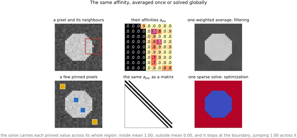
Hold the bilateral filter Tomasi & Manduchi 1998 in mind. To smooth a pixel $p$, it forms a weighted average of the neighbors $q$, where each weight, the affinity $a_{pq}$, is large when $p$ and $q$ are alike in value and small when an edge separates them. The output is that average, computed once, independently, for every pixel. Information crosses the image only as far as the filter's footprint reaches; a stroke of influence on one side of the picture has no way to reach the other in a single pass.
Neighboring residuals couple the unknowns across the image. On a connected region, one scribble can therefore influence distant pixels. Weak affinities reduce propagation across a luminance edge; they do not establish that the two sides have different true colors. Equal-luminance color boundaries remain ambiguous.
The price is that we no longer have a closed-form output per pixel; we have a system of coupled equations. The reward, as we will see, is that the system is exactly the kind we already know how to solve, and that the coupling is precisely what lets a handful of user marks fill an entire photograph.
Consider a long region with almost constant luminance and only one color scribble near its left end. One local averaging pass can transmit the scribble only as far as its neighborhood reaches. In a global optimization, adjacent unknown colors are coupled throughout the region. The solution can therefore carry the constraint much farther, even though each individual equation is local. A strong luminance boundary weakens the coupling if the affinity was designed that way. An unmarked disconnected region still needs a constraint or a convention; the solver cannot infer its intended color merely by being global.
10.3.2 Colorization: the canonical demonstration⧉
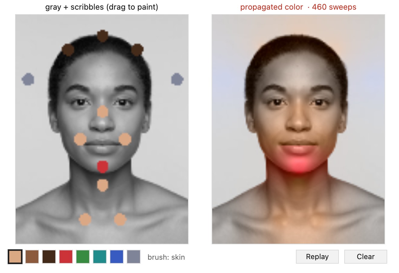
The crispest demonstration is colorization, due to Anat Levin, Dani Lischinski and Yair Weiss (2004). Start from a grayscale photograph, such as an old family portrait or a black-and-white film still, and the goal is to add plausible color. Doing it pixel by pixel would be hopeless. Instead the user scribbles a few coarse strokes of color roughly where each color belongs: a smear of red across the lips, blue on a sleeve, brown over the hair. The strokes need not be careful and need not fill anything; they are just hints. The algorithm then propagates the color from the scribbles to flood the rest of the image, under a single rule (Figure 10.3.1):
neighboring pixels of similar luminance should take similar color.
That rule is the bilateral's range idea stated verbatim: the same affinity, and the same idea that similar luminance means pixels belong together, but now expressed as something to minimize rather than average. It is a useful prior because many object boundaries coincide with luminance changes, while smooth shading often stays within an object. It can therefore propagate color without an explicit segmentation. It is still a prior: a shadow can create a luminance edge within one surface, and two different colors can meet at equal luminance. The user may need additional scribbles to resolve those cases.
The reason colorization is the canonical demonstration, rather than one application among many, is that it isolates the optimization idea cleanly. There is no clever color model, no segmentation, no learned prior. There is one quadratic energy, one affinity, and one linear solve, and yet a few seconds of scribbling colors an entire photograph. Everything edge-preserving and everything global about the method is on the surface.
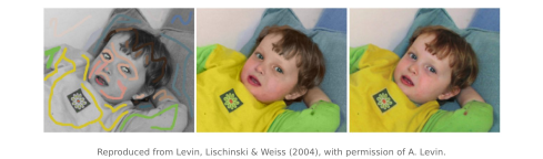
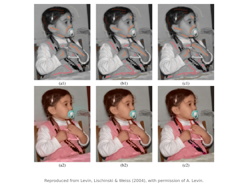
The original paper's own results show the method on photographs.
10.3.3 Writing down the energy⧉
We are given the luminance $I$ everywhere (it is just the grayscale image) and the user's scribbles at a few pixels. We solve for the chrominance $U$ (the color part, the two color-difference channels) at every pixel. Luminance is known; only color is unknown, which is why the energy is over $U$ alone.
The rule "each pixel's color should match the affinity-weighted average of its neighbors' colors" becomes, written as a penalty to minimize,
where $N(p)$ is the small neighborhood of pixel $p$ and $a_{pq}$ is the affinity between $p$ and its neighbor $q$. Each summand is one pixel's deviation from its neighbors' weighted average, squared so that positive and negative deviations both cost and so that the whole thing is a clean quadratic. Minimizing it drives every pixel toward agreement with the neighbors it most belongs with.
Two details make the term mean exactly what we said. First, the affinity is large when $I_p \approx I_q$ in luminance and small across a luminance edge: that is the entire edge-preserving content, the L10.1 affinity keyed on intensity difference. Second, the affinities around each pixel are row-normalized, $\sum_{q\in N(p)} a_{pq} = 1$, so that the inner sum $\sum_{q} a_{pq} U_q$ is a genuine weighted average of the neighbors rather than a mere weighted sum. With both in place, read the term back: each pixel's color should equal the affinity-weighted average of its neighbors' colors.
A natural choice for the affinity, and the one in the original method, makes the dependence on luminance difference concrete:
normalized over $q \in N(p)$, where $\sigma_p$ is a local measure of how much luminance varies around $p$ (so the falloff adapts to each region's contrast). This is the same exponential-of-squared-difference that gave the bilateral its range weight; here it is the same number doing the same job inside an energy. Where luminance is flat, neighboring $I$ values are close, the exponent is near zero, and the affinity is strong. Color couples tightly and flows freely, flooding the region. Where luminance jumps at an object boundary, $(I_p - I_q)^2$ is large, the affinity collapses toward zero, the coupling weakens, and color halts. A strong luminance boundary can therefore reduce spill from red lips onto the chin; it does not guarantee that every color boundary will be respected. (Levin and colleagues note that a correlation-based affinity works comparably; the exponential form is the cleanest to picture.)
Finally, the scribbles. They enter as hard constraints: at every scribbled pixel, $U$ is fixed to the color the user painted, and the minimization runs over only the unscribbled pixels. Those fixed values are what the propagation propagates: they pin the color at a few locations, and the energy carries it everywhere else along the high-affinity paths. (One could instead add a soft penalty pulling scribbled pixels toward the user's color; the hard-constraint version is simplest to state and is what the figure shows.)
The energy looks like it is asking for smoothness (every pixel near the average of its neighbors), and it is, but a very particular, edge-aware smoothness. A plain smoothness penalty would write $\sum_p \sum_{q\in N(p)} (U_p - U_q)^2$ with equal weight on every neighbor pair, which smooths across everything, edges included, and would smear color straight over object boundaries. Inserting the affinity $a_{pq}$ as the weight is the whole fix: pairs separated by a luminance edge carry almost no weight, so the solver pays almost nothing to let their colors differ, and the smoothing simply switches off across edges. This is the same move that turned the box average into the bilateral: weight the combination by belonging, transplanted from a filtering pass into the smoothness term of an energy. "Match your neighbors' weighted average" and "smooth, but not across edges" are the same instruction.
10.3.4 Solving it: a sparse linear system we already own⧉
Write $A_{pq}=a_{pq}$ and $B=I_n-A$, where $I_n$ is the identity matrix. The energy is $\|BU\|^2$. Partition columns into free and constrained pixels, $B=[B_F\ B_C]$, and let $U_C$ be the scribbled values. Then solve
The normal matrix is symmetric positive semidefinite. It is positive definite only when the constraints remove its nullspace. Constrain every otherwise free connected component or add a stated fidelity term. A row-normalized affinity matrix itself is generally not symmetric.
Each residual touches a small neighborhood. Its normal matrix can connect pixels that share a residual, so the stencil is wider than the original neighbor set. Apply the factors without explicitly forming the normal matrix when appropriate; least-squares solvers can also avoid squaring the condition number.
So the same toolkit applies, the machinery of Chapter 6.9, Efficient linear solvers:
- Conjugate gradient (CG), optionally preconditioned, the workhorse for a sparse, symmetric, positive-definite system like this one; it only ever needs to apply the operator to a vector.
- Multigrid, coarse-to-fine, which is especially apt here because color must travel long distances from a few scribbles, and solving on a small image first then refining propagates that long-range information far faster than iterating at full resolution.
These are the same tools that solve the Poisson equation for gradient-domain editing and that will solve the matting system in Part 19, Layers, transparency, compositing, and matting. The solver concepts transfer across these applications. Their operators and constraints still differ, so their nullspaces, conditioning and suitable preconditioners must be checked separately.
10.3.5 One affinity, two faces: the matting Laplacian connection⧉
The matting Laplacian Levin, Lischinski & Weiss 2008 (closed-form matting) is another sparse quadratic operator derived from local image statistics. It is not the same matrix as the row-normalized colorization affinity or its least-squares normal matrix. Chapter 10.5, Matting Laplacian derives its local affine color model.
The same energy template powers more than these two. Lischinski and colleagues Lischinski et al. 2006 used precisely this construction for interactive tonal and exposure editing: scribble "brighter here, darker there," and the affinity-weighted solve propagates a smooth, edge-respecting adjustment map across the photograph, so an exposure tweak floods a region and stops at its borders exactly as color does in colorization. In every case the recipe is the same: the user marks a few pixels, an affinity-weighted energy propagates the marks along smooth-luminance paths, a sparse solve fills the rest. Colorization is the cleanest face of a single, widely reused idea.
Everything above is an interactive method: the user supplies the scribbles, and a hand-built affinity prior carries them. The learned alternative dispenses with the scribbles entirely. Instead, train a CNN to predict plausible colors directly from a gray image (Zhang, Isola & Efros 2016), replacing the hand-designed affinity prior with one learned from millions of color photographs. That is the same "learned prior supersedes the hand-built one" move (Chapter 7.3, Deep learning, Chapter 7.4, Generative AI and diffusion) that overtakes denoising, deblurring, and inpainting, but the skeleton never changes: it is always data-fit + prior; this chapter has only shown what the prior looks like when it is an affinity and the solve is one sparse system.