18.2 Global tone mapping🔗⧉

A bright window and a dim room can both contain detail in a radiance map, yet be difficult to show together on a screen. A global tone map is the simplest answer: one curve, applied to every pixel, that takes scene luminance to display luminance. It can reveal information already captured, but cannot recover a clipped sensor measurement.

The curves of Chapter 8.3, Tone point operations already map input tones to output tones. Here the input is a radiance map with far more range than the output, and the curve has to compress it while keeping useful contrast. This chapter covers the classic global operators, from a single scale factor to curves shaped by the image's own histogram, and ends with the reason none of them can be the whole answer.

18.2.1 Two families: global and local🔗⧉

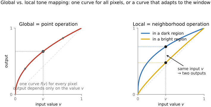
Scaling every value by the same factor preserves the scene's ratios, so it cannot by itself make a large range fit a smaller one (Chapter 17.1, Dynamic range and multiple-exposure capture); something has to compress. There are two fundamentally different ways to compress the range, global and local; this chapter covers the first and the rest of the part the second (Figure 18.2.1⛶ fullscreen).

A global tone map applies one function $L_\text{out}=f(L_\text{in})$ everywhere. A monotone scalar curve cannot create a new spatial maximum or minimum, so it does not generate the edge halos caused by a neighborhood filter. It can still reveal existing halos, amplify noise, produce banding after quantization, or alter colors. Compressing a large range reduces contrast over some input intervals.

A global curve redistributes contrast across intensities. For a small difference, $\Delta L_{\rm out}\approx f'(L)\Delta L$. For small relative contrast, the relevant gain is

A compressive log slope below one reduces relative contrast in that intensity range. The curve can allocate more contrast to populated or important ranges and compress others; it need not flatten every detail equally. The same input intensity still receives the same output regardless of its neighborhood.

A local tone map adapts to the neighborhood. One construction separates large-scale brightness from detail, compresses the former, and restores the latter. This can preserve texture while reducing the difference between a window and a wall, but the separation can mistake noise for detail and blur across boundaries.

18.2.2 Scale factors and logarithms: Ward and Drago🔗⧉

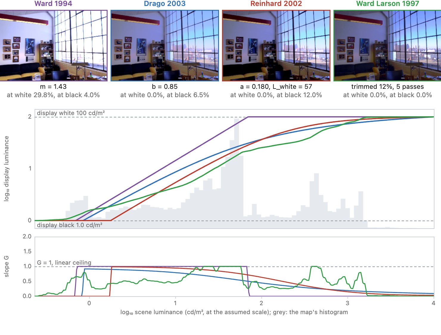
The simplest perceptually motivated operator is a single scale factor. Ward chose it so that a luminance difference that is just noticeable in the scene, at the scene's adaptation level, maps to a difference that is just noticeable on the display, at the display's adaptation level, using Blackwell's model of contrast thresholds Ward 1994 (contrast-based scale factor). With $L_{wa}$ the scene's adaptation luminance, for example its log average, and $L_{d,\max}$ the display's maximum, assumed to be viewed at an adaptation of half its maximum, the scale factor is

Being linear, it preserves every ratio and keeps threshold contrasts visible at the adaptation level, which suits scenes of moderate range; for a high-dynamic-range scene it clips the highlights, since a scale factor cannot compress.

Drago and colleagues compress with a logarithm whose base adapts to the luminance Drago et al. 2003. A logarithm in base 10 compresses strongly and suits the highlights; base 2 compresses less and keeps contrast in the shadows. Their operator interpolates the base from 2 in the darkest tones to 10 at the scene's maximum $L_{w,\max}$, with a bias exponent controlling where the transition happens:

with a bias $b$ around 0.85. It is fast, has one meaningful parameter, and handles a wide range without clipping. Like every curve in this chapter, it trades local contrast for range the same way at every pixel of a given luminance.

Figure 18.2.2⛶ fullscreen runs one radiance map through these two operators and the two of the next sections, Reinhard's and histogram adjustment, and plots each curve with its gain $G$.

18.2.3 One curve for everything: Reinhard's photographic operator🔗⧉

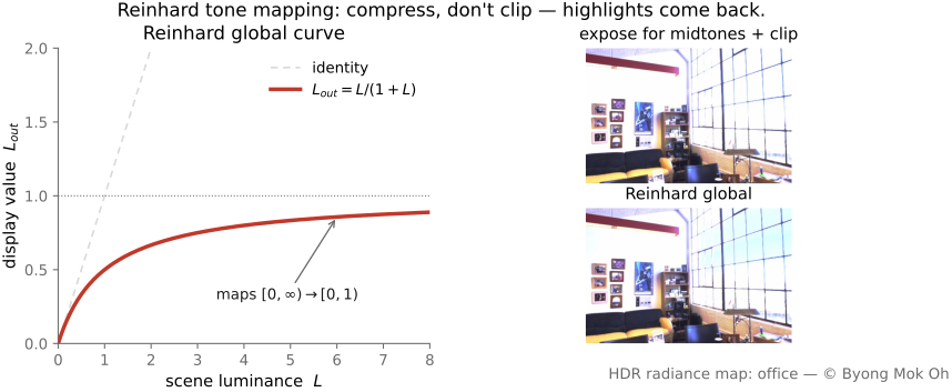
Clipping maps all values above the output limit to the same white. Scaling the maximum to that limit preserves distinctions among highlights but may leave most of the image too dark. A nonlinear curve can allocate more output range to dark and middle tones while compressing the highlights.

Reinhard et al.'s photographic operator Reinhard et al. 2002 begins by choosing an exposure scale. For nonnegative scene luminances $Y_i$,

The small positive $\delta$ permits black pixels; $a$ places the log-average before compression. Then apply

In words: take the scene luminance $L$ (which can run from 0 up to any large value) and send it through $L/(1+L)$. Read off the two ends. When $L$ is small, the denominator is near 1, so $L_\text{out} \approx L$, dark tones pass through almost unchanged, shadow contrast preserved. When $L$ is large, $L_\text{out} \approx 1$, the brightest highlights are gently drawn toward 1 but never quite reach it, so they roll off rather than clip. The entire infinite range $[0, \infty)$ maps smoothly into $[0, 1)$, with no hard clip anywhere (Figure 18.2.3⛶ fullscreen). A common variant takes a white-point parameter $L_\text{white}$, the luminance you want mapped exactly to 1:

A finite $L_\text{white}$ maps that value to 1, but values above it exceed 1; it is not an asymptote. All these luminances use the exposure scale defined above. For RGB, compute the mapped luminance $Y_\text{out}$ and multiply all channels by $Y_\text{out}/Y$ for $Y>0$, mapping black to black. This preserves RGB ratios before gamut mapping. It does not guarantee constant perceived hue or that each channel fits the output gamut. The result is display-linear RGB, to which we then apply the output encoding.

The white-point variant has a property worth knowing: near white its contrast gain $G$ exceeds one, up to about two for a low white point, so it adds contrast in the brightest tones rather than compressing them.

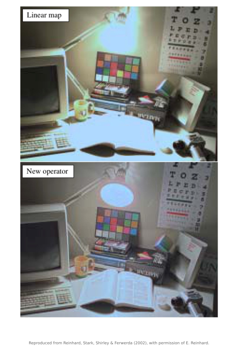
The key value is an exposure control, not the final displayed middle gray: $a$ becomes $a/(1+a)$ under the basic curve. A value such as 0.18 is a starting point, not an automatic exposure requirement.

The operator's own paper, which framed the whole method as digital photographic printing, makes both the curve and its key parameter concrete.

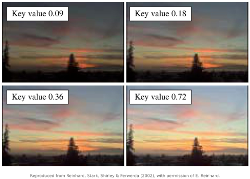
Reinhard is a compact example of global compression. Gamma and log curves also change relative contrast, while an S-curve can increase midtone contrast and compress both ends. The appropriate curve depends on the scene and the desired appearance; the beauty-curve chapter discusses that choice.

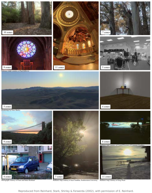
The same operator, with the same parameters, holds up across very different scenes, which is much of why it became the default global curve.

18.2.4 Histogram adjustment: a curve shaped by the image🔗⧉

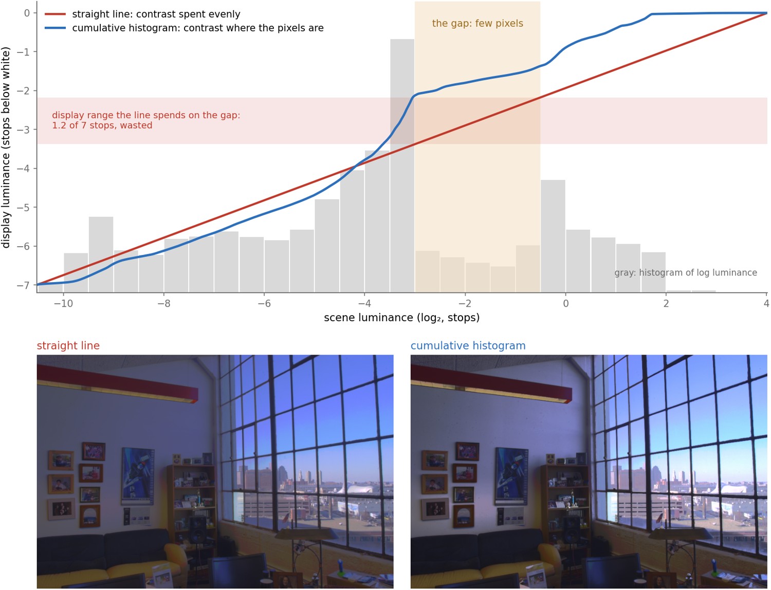
The display has a limited budget of contrast: its few stops of range, to be divided among the intensities of the scene. A curve that is steep over some range of scene luminance gives those intensities a lot of contrast, so their differences stay visible; a curve that is flat there merges them. Now look at the histogram of a high-dynamic-range scene in log luminance (Figure 18.2.7⛶ fullscreen). It is rarely spread evenly. An interior with a window has a large mound for the walls and furniture, a smaller one far to the right for the view outside, and comparatively few pixels in between: the intensities between the brightest wall and the darkest part of the window are present in a small fraction of the image, about a tenth in the office of the figure. A curve that spends contrast evenly across the whole range, a straight line in log-log coordinates, gives that sparse gap as much of the display's range as the walls, and those stops are largely wasted, since little there needs them. It is better to make the curve flat across the gap and steep where the pixels are, so that the walls and the view each get most of the range they need.

That is the idea of histogram-based tone mapping: allocate display contrast according to the image's intensity distribution. Larson, Rushmeier and Piatko constrain histogram adjustment using a visibility model (Ward et al. 1997).

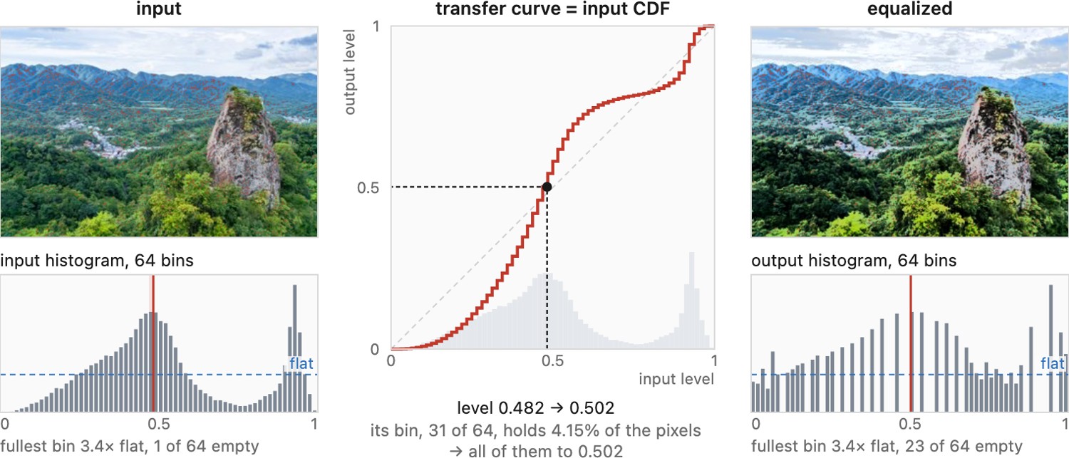
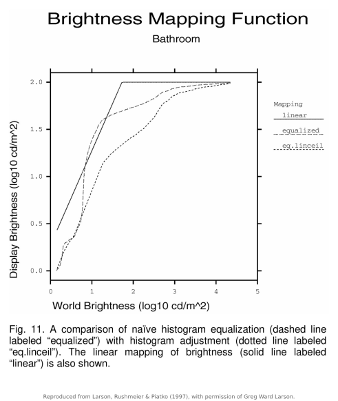
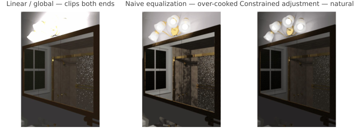
The method begins from a familiar image-processing reflex: histogram equalization, introduced in Chapter 8.7, Histograms for ordinary images (Figure 8.7.5⛶ fullscreen). We build the histogram of the scene's (log) luminances, then make the tone curve the cumulative distribution of that histogram. Where many pixels cluster (the mid-tones of a typical room) the curve is steep, spending lots of display range and so lots of contrast; where the histogram is sparse (the empty gulf between a dark interior and a bright window) the curve is flat, spending almost nothing. Adapting the curve to the image's own statistics is exactly the right instinct: the bins the scene populates get the contrast, the bins it doesn't are compressed away. But taken naively it overshoots badly. A heavily-populated bin earns a curve slope greater than one, which amplifies contrast there, exaggerating noise and pushing a flat wall or a patch of sky into a contrast it never had, an artificial, over-cooked look (the histeq panel below).

Their constraint is a cap on the slope of the tone curve. In log luminance, the equalized curve's slope at a given luminance is proportional to the histogram count there, so a crowded bin gets a steep curve. Larson and colleagues require that slope never exceed what the eye's contrast discrimination allows: a luminance difference that is just visible in the scene, at the scene's adaptation level, may map to at most a just-visible difference on the display, at the display's adaptation level. In the simplest version, which assumes Weber's law at both ends, the cap is a slope of one in log-log coordinates: the display never shows more contrast than the scene had. The published method replaces Weber's law with a threshold-versus-intensity function, which makes the cap vary with brightness and can let it exceed one. The eye's threshold contrast grows as luminance falls, so where the display shows a pixel dimmer than the scene did, a just-visible difference needs more contrast on the display than in the scene, and the cap allows it: at the default settings of Figure 18.2.8⛶ fullscreen, slopes reach about 2.6. When the cap cannot be met at all, as in very dim scenes, the method falls back to a linear map.

Figure 18.2.8⛶ fullscreen follows the method step by step on a radiance map, from the histogram and its equalization curve to the ceiling, the trimming and the final curve.

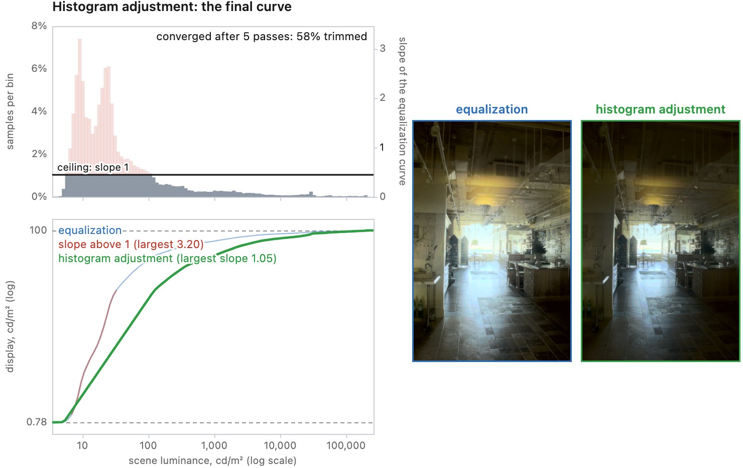
The procedure turns the cap into a limit on each histogram bin and enforces it by trimming:

b = histogram(log(L_foveal), bins)          # luminance sampled about once per degree of view
total0 = sum(b)
repeat:
    ceiling = count_limit_from_slope_cap(b)  # the most a bin may hold, given the current total
    trimmed = sum(max(b - ceiling, 0))
    b = min(b, ceiling)
until trimmed < 0.025 * total0             # the paper stops once a pass trims under 2.5% of the original count
curve = cumulative(b) / sum(b)              # maps log scene luminance to log display luminance

Trimming lowers the total, which lowers every bin's ceiling, which is why it iterates. The curve keeps equalization's adaptivity, spending display range where the scene's values are, while the cap prevents it from manufacturing contrast beyond the model's visibility limit in the crowded bins. That is a perceptually motivated model, not a guarantee that the output never enhances noise or looks objectionable: it depends on the assumed adaptation levels and viewing conditions.

The trimming stage of Figure 18.2.8⛶ fullscreen runs this loop one pass at a time.

Figure 8.7.13⛶ fullscreen overlays the three curves: the straight line that ignores the histogram, equalization with its slopes above one, and histogram adjustment, which follows equalization's shape with every slope clipped.

The result is still one curve. Two pixels of equal luminance get the same output whatever surrounds them, so histogram adjustment still trades global range against local detail, only more carefully than a fixed gamma or shoulder. Keeping local contrast while compressing range requires a mapping that depends on each pixel's neighborhood, the local methods of the following chapters. A fair comparison puts it beside a simpler curve and a local operator under the same display conditions (Chapter 8.7, Histograms).

Figure 8.7.12⛶ fullscreen shows the three renderings side by side; the operator is first built in Chapter 8.7, Histograms, where the same figures appear.

18.2.5 Why log space helps🔗⧉

Log luminance makes relative contrast convenient to manipulate. Scaling a log difference by $c$ changes the corresponding luminance ratio $R$ to $R^c$. For $0<c<1$, this compresses the ratio. Multiplication in linear light is already simple; the benefit here is that ratios become differences that can be separated into base and detail.

This is why the local methods of the following chapters work on log luminance: a base and a detail layer of the log image are a large-scale ratio and a local ratio, and compressing the base compresses large ratios while leaving local ones alone (Chapter 18.3, Two-scale and bilateral tone mapping).

18.2.6 From luminance to color🔗⧉

Most operators in this part compute a new luminance and leave the color to a separate rule. With linear RGB $c$ and positive luminance $L$, scaling by $L_{\rm out}/L$ preserves RGB ratios before clipping:

Very small or nonpositive luminances need a guard, and gamut excursions need inspection. Preserving linear RGB ratios does not guarantee constant perceived hue or saturation after display mapping. Applying separate nonlinear curves to channels changes those ratios. The chosen color space and gamut treatment should be stated with the result. The alternative, applying the curve to each channel separately, desaturates bright colors toward white, which is sometimes wanted and sometimes not; Chapter 18.8, Display rendering transforms and color treats the choice in detail.

18.2.7 Why a single curve cannot win🔗⧉

At a given input level, a global curve gives every pixel the same adjustment. If a window and a wall require different treatments at that level, one curve cannot supply them. A local operator can, at the cost of neighborhood-dependent artifacts and more parameters.

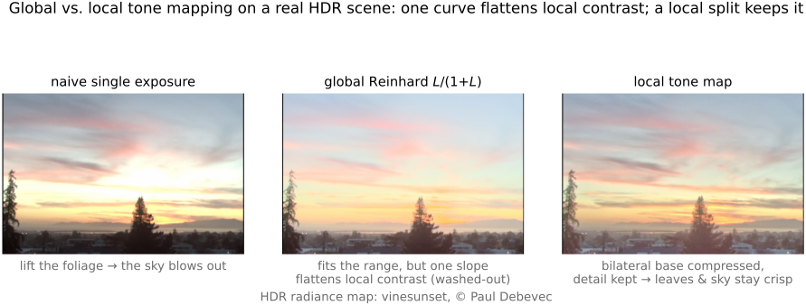
Consider a dark textured wall and a bright textured cloud. A global curve must assign the same output and the same local slope whenever their input values coincide. Flattening a broad part of the curve to fit the scene range also reduces small variations that fall in that part. A local method can treat the wall and cloud differently by using their neighborhoods, but then the transition between neighborhoods becomes part of the problem. The global/local choice trades one consistent mapping for spatial flexibility; it does not make range compression free.

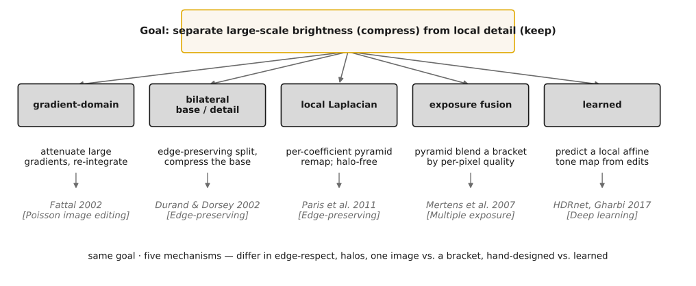
The argument can be made exact with the gain $G(L)$ of the two-families section. A curve that compresses a range of $R$ stops into $r<R$ has an average log-log slope of $r/R$, so over most of the range it must reduce relative contrast, and a small texture at any luminance in that range is reduced along with the large difference that had to be compressed. No choice of shape escapes this, since the curve sees only the value, not whether a variation is the edge of a window or the grain of a wall. Keeping local contrast while compressing the range needs spatial processing: a mapping that depends on each pixel's neighborhood. The rest of the part develops the five ways of doing that (Figure 18.2.10⛶ fullscreen).

18.2.8 Choosing and checking a tone map🔗⧉

We start by checking whether the recorded highlights contain usable detail and whether the shadows contain signal above noise. Choose output brightness and contrast for the destination. A global curve is inexpensive and easy to inspect; add local adjustment when regions need different treatment. We then check strong edges for halos and flat shadows for amplified noise, at viewing size and in a pixel-level crop.

Camera looks and raw-developer defaults encode choices of curve and of local adjustment. They are best compared at a common output brightness and size, looking at faces, skies, saturated highlights and dark texture. A rendering with more visible detail is not automatically the better photograph.