33.2 Compressive sensing⧉
Here is a fact that should sound impossible. Suppose the scene has a million unknowns, a megapixel image, and you take only fifty thousand measurements, each one a single number that mixes the entire scene together. I have thrown away nineteen out of every twenty degrees of freedom before the data even reaches you. By the bookkeeping of Chapter 7.1, Imaging as Bayesian inference with probabilistic priors you are sunk: the operator is wildly underdetermined, its null space is enormous, and infinitely many scenes produce exactly the measurements you hold. For a sufficiently sparse signal, a suitable random measurement ensemble, enough measurements, and noiseless data, exact recovery can be guaranteed with high probability. Sparse and random alone are not sufficient. That is the claim of compressive sensing (also called compressed sensing), and when Candès, Romberg & Tao and, independently, Donoho proved it in 2006 it surprised the field [@candes-romberg-tao-2006; @donoho-2006].
It earns a chapter because it is the part's central move stated in its purest form. The optics encode: a designed operator $A$ folds the whole scene down into a short list of coded measurements, a code that is emphatically not yet a picture. The computation decodes: it reconstructs the full scene from that short list. There is no blur to invert, no depth to read out, nothing but the bare encode→decode pair. That is exactly why it belongs here, and why we lead with it before the messier optical codes.
33.2.1 Sub-Nyquist: fewer measurements than unknowns⧉
Start with the wall compressive sensing walks through. The classical rule for how much you must sample is Nyquist's: to capture a signal band-limited to some maximum frequency, you must sample at twice that frequency, or you lose information irrecoverably to aliasing (Chapter 6.3, Linearity, Fourier, Aliasing and deblurring; Shannon 1948 Shannon 1948). Nyquist is a worst-case promise: it assumes the signal could have anything up to its band limit, and under that assumption it is tight: you genuinely cannot do with fewer samples.
But most real signals are nowhere near worst-case. A photograph is not arbitrary million-dimensional static; it is mostly smooth regions and a few edges, and in a wavelet or DCT basis the overwhelming majority of its coefficients are essentially zero. That is exactly the fact that makes JPEG work: transform the image, keep the few big coefficients, throw the rest away, and the picture survives. Call a signal $k$-sparse if, in some known basis, only $k$ of its $n$ coefficients are nonzero; a signal with a small tail of other coefficients is called compressible, with $k \ll n$. The whole point of compression is that natural signals are highly sparse: a megapixel image might be well approximated by a few tens of thousands of wavelet coefficients.
Now ask the question that launches the field. Compression means measuring everything and then throwing most of it away: capture all $n$ samples, transform them, and discard most coefficients. If the signal really only has $k$ degrees of freedom, why did we ever measure $n$ of them? Why not capture just the information we are going to keep, and skip the wasteful step of measuring a million numbers to retain fifty thousand? Compressive sensing answers: you can, and you do not even need to know which coefficients are the big ones in advance. The remaining question is how you measure.
33.2.2 Two ingredients: incoherent measurements and sparsity⧉
The method has two ingredients, and they work for complementary reasons.
The first ingredient is the measurement operator, and the surprising design rule is: make it random. Each row of $A$ is a random pattern, such as random signs, Gaussian weights, or a random binary mask, and each measurement $y_i = A_i \cdot \mathbf{x}$ is the inner product of that random pattern with the whole scene. So every single measurement is a coded sum that touches every pixel at once, scrambled by random weights. This is the opposite of an ordinary camera, where pixel $i$ measures scene location $i$ and nothing else. The technical word for what we want is incoherence: the measurement patterns must be spread out, dense and unstructured, in whatever basis the signal is sparse in. A sparse signal is concentrated (a few big coefficients); incoherent measurements are maximally spread (every measurement smears all coefficients together). When a concentrated thing is measured by spread-out patterns, each measurement carries a little information about every coefficient, and no coefficient can hide. Suitable normalized random ensembles have favorable properties relative to a fixed sparsifying basis with high probability. Arbitrary random matrices, uncentered binary masks, and constrained optical operators need separate analysis. You do not need to know where the signal is sparse, only that it is.
The second ingredient is the sparsity prior, and it is what breaks the underdetermination. The system $A\mathbf{x} = \mathbf{y}$ is wide: infinitely many $\mathbf{x}$ satisfy it, a whole null space worth. Among all of them, compressive sensing picks the sparsest one, the one with the fewest nonzero coefficients. The bet is that the true signal is sparse and the decoys threaded through the null space are not, so "sparsest" singles out the truth. This is the same logic as every inverse problem in the book: of all scenes consistent with the data, choose the one the prior prefers (Chapter 7.1, Imaging as Bayesian inference with probabilistic priors). Here the prior is sparsity. What is special is how cleanly it works: with the right $A$, sparsity does not merely prefer the right answer, it pins it down uniquely and exactly.
How many measurements do you need? Not $n$, and not merely $k$, but a small multiple in between: roughly
random measurements suffice to recover a $k$-sparse signal of length $n$, where the constant and probability bounds depend on the matrix ensemble and recovery conditions. In noisy data, approximate sparsity yields an error bound rather than exact recovery. Read it in words: you pay for the number of nonzero coefficients $k$ (the signal's true complexity), plus a logarithmic overhead $\log(n/k)$ that is the price of not knowing in advance which coefficients are the nonzero ones. The randomness buys you that ignorance cheaply. For a signal that is $5\%$ sparse, this is a large saving over measuring all $n$.
33.2.3 Recovery by $\ell_1$: the geometry of basis pursuit⧉
The decoder has to solve an underdetermined system by finding the sparsest solution. The plain statement of "sparsest" counts nonzeros, the $\ell_0$ "norm," $\lVert\mathbf{x}\rVert_0$ = number of nonzero entries, and minimizing it directly is a combinatorial nightmare: you would have to try every subset of coefficients, which is NP-hard and hopeless at image scale. So the naive exact objective is computationally impractical.
But you do not need it. Replace the count of nonzeros, $\ell_0$, with the sum of absolute values, the $\ell_1$ norm $\lVert\mathbf{x}\rVert_1 = \sum_i |x_i|$, and solve
This is a convex problem (a linear program, in fact) that is solvable efficiently and at scale, and it is called basis pursuit. The key result is that, under the right conditions on $A$, minimizing the convex $\ell_1$ surrogate returns exactly the same answer as minimizing the intractable $\ell_0$ count. You get the genuinely sparsest solution by solving an easy problem instead of an impossible one.
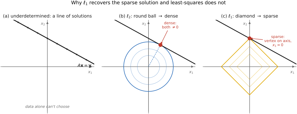
Why does $\ell_1$ favor sparsity when its obvious cousin $\ell_2$ (ordinary least-squares, the minimum-energy solution) does not? The answer is geometry, and it recurs everywhere sparsity appears in this book (Figure 33.2.1). The constraint $A\mathbf{x}=\mathbf{y}$ is an affine set, a line in a 2-D cartoon. To minimize a norm subject to that constraint, you inflate the norm's unit ball from the origin until it just touches the constraint line; the touch point is the answer. The $\ell_2$ ball is a sphere, perfectly round, so it generically first touches the line at a generic point: a solution with all coordinates nonzero, dense. The $\ell_1$ ball is a cross-polytope: a diamond in 2-D, an octahedron in 3-D, sharp spikes poking out along the coordinate axes. An inflating diamond almost always touches a tilted line at one of its vertices. A vertex sits on an axis, meaning the other coordinates are exactly zero. The sharp corners of the $\ell_1$ ball are pointed precisely at the sparse solutions; the round $\ell_2$ ball has no such corners and slides to a dense one. That is the intuition for why $\ell_1$ recovers sparsity and $\ell_2$ does not.
In practice the measurements carry noise, so we do not insist on $A\mathbf{x}=\mathbf{y}$ exactly. We relax the equality into a data-fit penalty and solve the LASSO:
which is, once again, exactly the book's universal recipe: data fit plus a prior (Chapter 7.1, Imaging as Bayesian inference with probabilistic priors), with the $\ell_1$ term as a sparsity-promoting regularizer and $\lambda$ trading the two off. When the signal is sparse not in the pixel basis but in a transform (wavelets, DCT), the $\ell_1$ penalty is applied to the coefficients (minimize $\lVert W\mathbf{x}\rVert_1$ for the wavelet transform $W$), which is the form used for images.
33.2.4 Why it works: the restricted isometry property, intuitively⧉
There is one condition on $A$ that makes the whole thing rigorous, and it has a clean intuition even though we will skip the proofs entirely. Call it the restricted isometry property, or RIP. An isometry is a map that preserves distances (a rotation, for example). We cannot ask a wide $A$ to be an isometry on all of the million-dimensional space; it is squashing a million numbers down to fifty thousand, so it must collapse most directions. A sufficiently strong RIP condition provides a useful sufficient recovery guarantee: that $A$ act like an isometry when restricted to sparse vectors. That is, for any two $k$-sparse signals, the distance between their measurements is close to the distance between the signals themselves: $A$ neither collapses two distinct sparse signals onto the same measurement nor stretches them wildly apart.
Since the difference of two $k$-sparse vectors is at most $2k$-sparse, distance preservation requires a condition at order $2k$. RIP is a sufficient route to stable recovery, not a necessary characterization of every recoverable operator. If $A$ keeps distinct sparse signals distinct after measurement, then the measurement uniquely identifies which sparse signal produced it. The encoding is invertible on the set of sparse signals, even though it is hopelessly non-invertible on the full space. And it is stable: because near sparse signals stay near, a little measurement noise moves the recovered signal only a little, instead of detonating the way naive inversion of an ill-conditioned operator does (Chapter 7.1, Imaging as Bayesian inference with probabilistic priors). The deep result is that random matrices satisfy the RIP with overwhelming probability once you have the $m \approx Ck\log(n/k)$ rows above, which is why "make it random" is not a hack but the heart of the method. Designing a deterministic matrix that provably satisfies RIP is hard; a suitable random construction gives such guarantees probabilistically, without making optical implementation or verification free.
33.2.5 The single-pixel camera⧉
The clearest embodiment of all this is a camera with one pixel (Figure 33.2.2). A camera with a single photodiode sensor sounds implausible, but it is a real instrument, built by Duarte and colleagues at Rice, and it photographs two-dimensional scenes Duarte et al. 2008. The trick is to put the coding in the optics and let computation do the rest.
The scene is imaged onto a digital micromirror device (DMD), the same chip used in DLP projectors, an array of a million tiny mirrors each of which can independently flip to "on" or "off" (it is one of the optical modulators the part covers in its own chapter, spatial light modulators). The mirrors set to "on" bounce their patch of the image toward a second lens that funnels all of that collected light onto the single photodiode. So the photodiode reads out one number: the sum of the scene over exactly the pixels the DMD turned on, which is precisely the inner product of the scene with a binary mask. Load a random binary pattern onto the DMD, take a reading: that is one random measurement $y_i = A_i\cdot\mathbf{x}$. Load a fresh random pattern, take another. After $m$ patterns you have $m$ coded measurements with $m \ll n$, and you reconstruct the full image by $\ell_1$ recovery in the wavelet basis. The DMD displays nonnegative binary masks. Complementary measurements can realize signed patterns by subtraction, at the cost of additional reads and noise; the DMD displays the physical rows of the measurement operator one at a time; the photodiode evaluates the inner products; the laptop decodes.
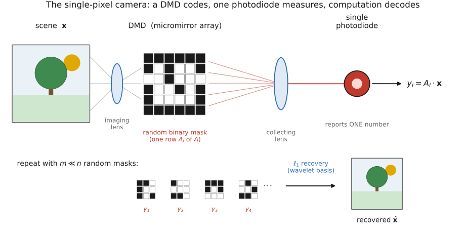
It is the encode→decode story with nothing left out: the optics form a code that is not a picture (a list of inner products against random masks), and computation turns the code into the picture. What it costs is time: you took $m$ measurements sequentially, one mask at a time, so a single photograph that an ordinary sensor grabs in one exposure now takes hundreds or thousands of sequential readings, during which the scene had better hold still. That cost is the hinge of the pointed question we close on.
33.2.6 Where compressive sensing wins, and where it does not⧉
It is tempting to read the single-pixel camera as the future of photography. It is not, and understanding why is the most useful thing this chapter can leave you with.
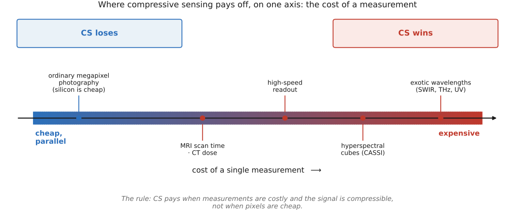
For ordinary visible-light photography, compressive sensing loses, and it loses for a blunt economic reason: silicon pixels are absurdly cheap. Mass-produced silicon arrays acquire many spatial samples in parallel at low cost per sample. There is simply nothing to save by measuring fewer of them: the wasteful "measure $n$, keep $k$" step that compressive sensing was invented to avoid is often much cheaper than sequential optical coding and reconstruction. Against a parallel megapixel sensor, the single-pixel camera's sequential coded measurements are slower, more fragile to motion, and more complex, for a recovered image that is no better. When pixels are cheap, just buy pixels.
Compressive sensing earns its keep exactly where a pixel is expensive, where you cannot simply throw down a cheap array of millions of detectors. That is a real and important set of regimes:
- Exotic wavelengths. Outside the visible, array sensors get costly or impractical fast: short-wave infrared, terahertz, some ultraviolet bands. A single detector at such a wavelength can be affordable where a megapixel array is not, and a single-pixel architecture with compressive sensing buys 2-D imaging from that one expensive detector.
- Hyperspectral imaging. Here you want a full spectrum at every pixel, a data cube far too large to sample densely, yet that cube is highly compressible. Coded-aperture snapshot spectral imagers (CASSI) put a coded mask and a disperser in the optics to multiplex the spectral cube onto a 2-D sensor in one shot, then reconstruct it by sparse recovery Wagadarikar et al. 2008.
- Medical imaging: MRI and CT. This is where compressive sensing made its largest real-world dent. An MRI scanner measures the image's Fourier coefficients one (expensive, slow) line at a time, and the cost is the patient's time in the bore; a CT scanner measures X-ray projections, and the cost is radiation dose. Measuring fewer coded lines or projections and reconstructing with a sparsity prior can reduce acquisition time or dose, but preservation of diagnostically important detail must be validated for the acquisition and reconstruction protocol; it is not guaranteed by a generic sparsity argument. The saving is paid in human terms, not dollars. Here the measurement, not the pixel, is the thing that is dear.
- High-speed imaging. When the bottleneck is how fast you can read pixels off the chip, taking fewer (coded) measurements per frame trades reconstruction for frame rate.
The common thread (Figure 33.2.3): compressive sensing replaces some measurements with stronger assumptions and more computation. It pays when each measurement is costly (in money, time, dose, or readout bandwidth) and the signal is compressible, so that buying a few clever coded measurements and decoding them beats buying many literal ones. It does not pay when measurements are already cheap and parallel, which is the entire regime of everyday digital photography. That is the fair place to leave it: a surprising idea that matters in a few imaging niches, but not in everyday phone photography.