10.4 Local Laplacian filters🔗⧉

Enhancing rock texture should not put a bright rim around a mountain silhouette. Local Laplacian filters control detail and large contrast through a pointwise remapping used to construct each output pyramid coefficient Paris et al. 2011.

The goal is simple. At every pixel and every scale, an image carries some amount of local contrast, how far this pixel departs from its blurred surroundings. Some of that contrast is detail (the rock grain, the pine needles): small departures we want to amplify. Some of it is an edge (the mountain against the sky): a large departure we want to leave exactly alone. Edge-aware detail manipulation is, at heart, nothing but the wish to grab the small departures and lift them while the large ones pass through untouched. The trouble has always been telling the two apart cleanly enough that the boundary between them does not itself become an artifact.

This chapter is one very clean answer, due to Sylvain Paris, Samuel Hasinoff and Jan Kautz (2011). It does not build a base layer and does not weigh any pair of pixels. Instead it processes a Laplacian pyramid (the multiscale decomposition of Chapter 6.6, Pyramids and wavelets) by reshaping each coefficient with a smooth point curve that is recomputed, per output pixel, to know whether that pixel sits on detail or on an edge. The pyramid uses ordinary blurring, but the remapping used to obtain each coefficient gives explicit control over small and large intensity differences. This substantially reduces the halos of naive coefficient manipulation. The same family of curves supports detail enhancement, tone mapping and inverse tone mapping; a sampled approximation makes the construction practical and connects it to the unnormalized bilateral filter Tomasi & Manduchi 1998.

10.4.1 The wish, and why the bilateral leaves a halo🔗⧉

Recall the two-scale story of Chapter 10.1, Bilateral filtering and Chapter 18.2, Global tone mapping. To manipulate detail or compress a high-dynamic-range (HDR) scene, the classic move is to split the image into a base (a piecewise-smooth, edge-respecting version that holds the large-scale tones) and a detail layer (everything the base threw away). You then squash the base to fit the display and add the detail back, often boosted. The base is built with an edge-preserving smoother (a bilateral filter, say) precisely so that the strong edges land in the base and do not get manipulated as if they were texture.

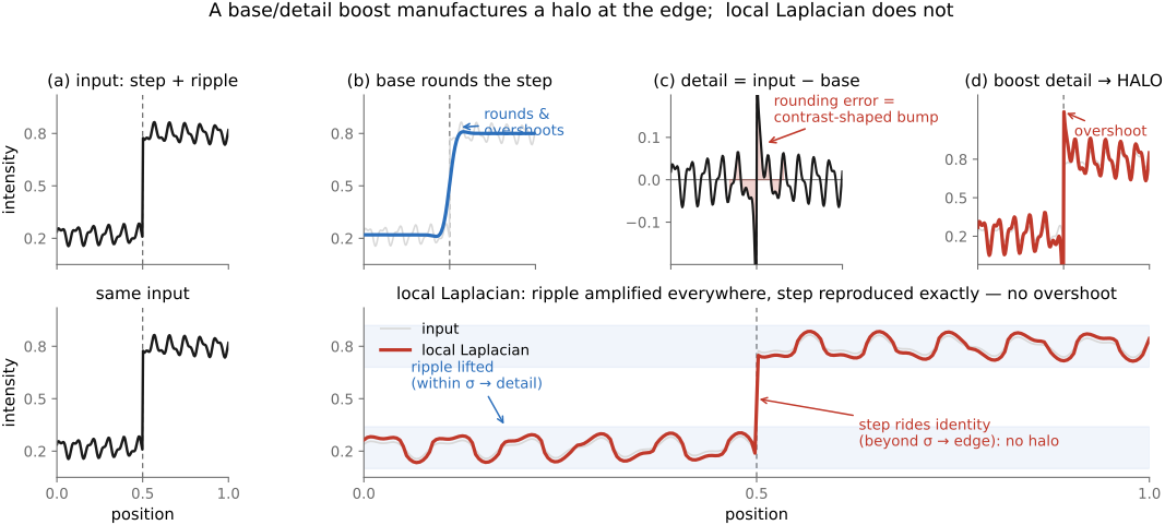
It works beautifully right up until the base is imperfect at the edge, and that is where halos come from. If the base layer rounds a sharp silhouette even a little (underestimating the bright side and overestimating the dark side) that error lands in the detail layer as a contrast-shaped bump straddling the edge. Boost the detail and you boost the bump: a glowing rim on one side, a dark trench on the other. Worse, push hard enough and a gradient can reverse: the detail layer's overshoot dominates and the slope across the edge flips, so a bright-to-dark edge reads locally as dark-to-bright. Halos and gradient reversals are the two failure modes that motivated the bilateral in the first place, and the bilateral merely reduces them; it does not abolish them, because the single base layer still has to commit, once, to one smoothed value at each pixel of the edge.

Local Laplacian filtering changes how the coefficients are constructed. The decision about which intensity differences to modify is made for each coefficient through a remapping curve, rather than through one base/detail split. This provides more control over the interaction between detail and strong edges (Figure 10.4.1⛶ fullscreen).

10.4.2 What a Laplacian pyramid hands you🔗⧉

Local Laplacian filtering is built directly on the Laplacian pyramid Burt & Adelson 1983 (Laplacian pyramid) of Chapter 6.6, Pyramids and wavelets, so recall exactly what that decomposition gives. Blur the image and subtract the blur from the original: what remains is the finest band, the contrast the blur removed, namely the texture and edges at the smallest scale. Now downsample the blurred image and repeat: each level $\ell$ holds the contrast at one scale, and the bottom of the pyramid holds the leftover low-frequency residual. Collapsing the pyramid (upsampling and adding the bands back) reconstructs the image exactly.

A Laplacian-pyramid coefficient $\ell_\ell(p)$ at level $\ell$ and pixel $p$ is the local contrast at that scale and place, how far $p$ departs from its blurred surroundings at that scale. Its magnitude is the natural measure of "detail versus edge": small coefficients are fine modulation we may want to lift; large coefficients are strong structure we want to preserve. So the wish from the opening (amplify small departures, leave large ones alone) translates cleanly into the pyramid: amplify small-magnitude coefficients, pass large-magnitude ones through.

The difficulty is that a coefficient arrives unlabeled. A coefficient of a given magnitude over a smooth region might be the fine texture we want to boost; a coefficient of the same magnitude sitting on the flank of a strong edge is part of that edge and must not be touched. The naive remedy ("amplify coefficients below some magnitude threshold and not above") is exactly the base/detail thresholding that halos: it makes a hard, per-coefficient cut with no regard for the pixel the coefficient belongs to, and the discontinuity at the threshold becomes the artifact. We need a decision that depends on the value of the pixel the coefficient is reporting on, and that is the move the next section makes.

10.4.3 The mechanism: a remapping recomputed per output pixel🔗⧉

For output coefficient $(\ell,p)$, use the reference value $g=G_\ell[I](p)$ from the input Gaussian pyramid at the same level and location. Remap the full-resolution input about $g$, construct its Laplacian pyramid, and take coefficient $(\ell,p)$. Repeat for the output coefficients and reconstruct using the matching pyramid expansion. Using the full-resolution value $I(p)$ at every level would be a different algorithm.

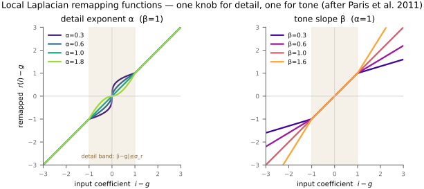
That sounds extravagant, and naively it is (we will address the cost at the end). But look at why it does the right thing. The curve $r_g$ is centered on $g$ and reshapes intensities by how far they sit from $g$:

For departures below $\sigma$, $\alpha<1$ enhances small differences and $\alpha>1$ suppresses them. For larger departures, $\beta$ controls the slope: $\beta=1$ retains them, $0<\beta<1$ compresses them, and $\beta>1$ expands them. Both branches meet at the threshold. Values very close to the reference need care when $\alpha<1$, because the power curve has a steep derivative and can amplify noise.

The remapping distinguishes departures relative to the local Gaussian reference. It can reduce the halos of a single blurred-base decomposition, but the argument is not that every coarse reference equals one side of an edge. Inspect the assembled multiscale result, especially at extreme parameters.

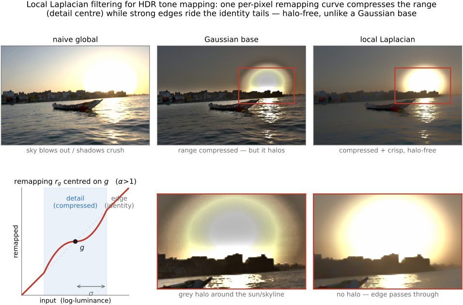
The computational expense follows directly from selecting one coefficient at a time. For the requested level and position, use the corresponding value in the original Gaussian pyramid as the remapping reference. Remap the input around that reference, construct the needed Laplacian coefficient, and copy it into the output pyramid. A different level or position generally selects a different reference and therefore a different remapping. The conceptual algorithm recomputes far more than the one coefficient it keeps, which motivates the later approximation using a finite set of reference intensities. This also explains why taking one globally remapped image and building its pyramid is a different operation.

10.4.4 One curve, three edits: enhancement, tone mapping, inverse tone mapping🔗⧉

Because the entire design lives in the shape of $r_g$, three different photographic operations are three settings of the same method, a clean instance of big lesson L10.4show, that the eye reads local contrast and not absolute level, so the right place to edit is the multiscale contrast itself.

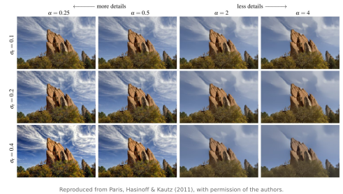
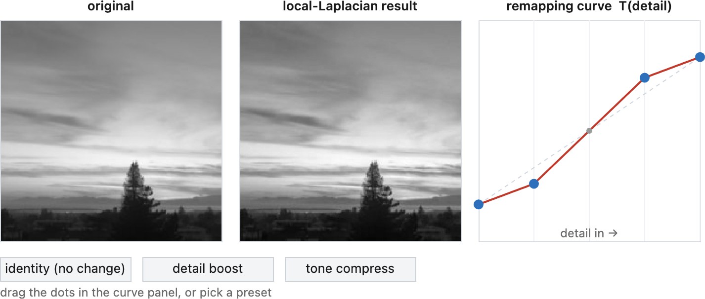
• Detail enhancement. Make the center of the curve steeper than the identity ($\alpha<1$): small departures from $g$ are stretched, so texture and fine local contrast leap out, while edges on the identity tails stay put. Set the large-departure slope to $\beta=1$ for this detail-enhancement setting, and limit amplification near zero to avoid lifting noise.

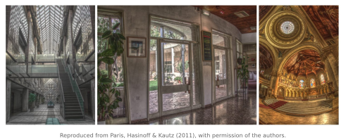
• HDR tone mapping. Compress large departures with $0<\beta<1$ while choosing $\alpha$ separately for detail. Suppressing small departures alone is not the intended dynamic-range control. State the input domain and final display mapping.

• Inverse tone mapping. Invert that compression (expand large-scale contrast) to take a flat or low-dynamic-range image and re-inflate its range, the operation you want when feeding standard-range content to an HDR display.

These settings change different ranges of contrast. They do not guarantee artifact-free output or recover radiance lost to clipping. Noise, strong parameter settings and finite intensity sampling remain practical limitations.

10.4.5 Contrast with the bilateral base/detail split🔗⧉

This differs from the bilateral approach in one specific way, though both aim at the same target. The bilateral two-scale decomposition (Chapter 10.1, Bilateral filtering, Chapter 18.2, Global tone mapping) and local Laplacian filtering share the goal of compressing the range or boosting detail without halos, and they are formal cousins. They part on the machinery.

The bilateral route is affinity-based and once-committing: it measures how similar nearby pixels are (the range weight), averages the similar ones into a single base layer, and then manipulates the detail = input − base. Every pixel of the edge gets one smoothed base value, and any imperfection in that one commitment becomes a halo in the boosted detail.

Local Laplacian filtering constructs coefficients using remappings centered at Gaussian-pyramid values. The pyramid still uses blurring and a coarse residual; the distinction is how each coefficient is chosen, not the absence of a base or averaging at all scales.

10.4.6 The cost, and the fast version🔗⧉

The plain catch is cost, and reading the recipe back makes it clear: the naive filter rebuilds an entire Laplacian pyramid per output pixel and per level, which is wildly redundant. Most of each rebuilt pyramid is thrown away after one coefficient is read. Done literally, that is far too slow for a real photo.

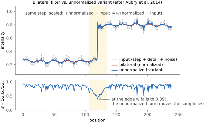
The fast version, Mathieu Aubry, Sylvain Paris, Samuel Hasinoff, Jan Kautz and Frédo Durand (2014), recovers practicality with two observations. The first is sheer efficiency: the remapping $r_g$ depends on $g$ only through a smooth dependence on the center value, so it suffices to evaluate the construction for a small handful of representative values of $g$ spanning the intensity range and interpolate between the resulting pyramids, turning a per-pixel rebuild into a few full-image pyramids plus a lookup. The second is conceptual, and it is the one this book cares about most: the single-scale special case of the local-Laplacian construction is exactly the unnormalized bilateral filter from the end of Chapter 10.1, Bilateral filtering, the delta-from-input form

This connection requires matching kernels, remappings and normalization conventions; it is not an identity for every choice of local-Laplacian curve and bilateral weights. The explicit step size here follows Chapter 10.1, Bilateral filtering.

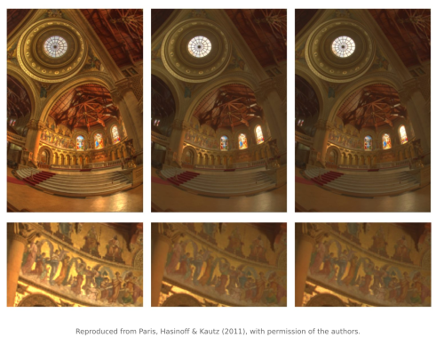
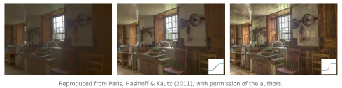
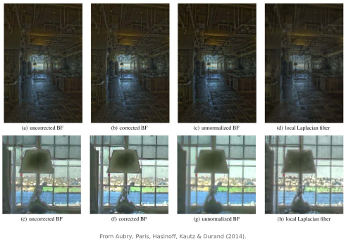
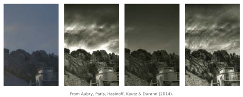
With the filter now fast, the authors put it through the photographic operations the slow version promised, at full image resolution. The first is the hardest test of the whole approach: range compression and detail enhancement at once, in a single pass.

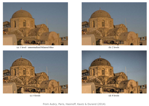
The remaining results probe what the dials actually do once the filter is cheap enough to sweep them. The most structural dial is the depth of the pyramid, how many scales the remapping is allowed to touch.

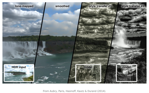
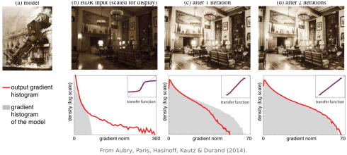
Because the filter acts on coefficients, it can also be driven toward a target rather than a fixed curve, iterating the remapping until a desired statistic of the result is met.