16.9 Measuring a deblur⧉
Levin et al. examined estimator behavior and evaluation using controlled blur data (Levin et al. 2009). A central practical lesson is to separate the quality of a kernel estimate from the behavior of the non-blind solver that consumes it.
A comparison can answer either which kernel estimator is better or which complete system produces a better image. State which question is being tested.
16.9.1 What went wrong, specifically⧉
Three things, each ordinary on its own.
Synthetic kernels test a specified family. Measured trajectories add realistic motion patterns, but do not capture every spatially varying blur, optical effect or saturation condition. Include data representing the intended use.
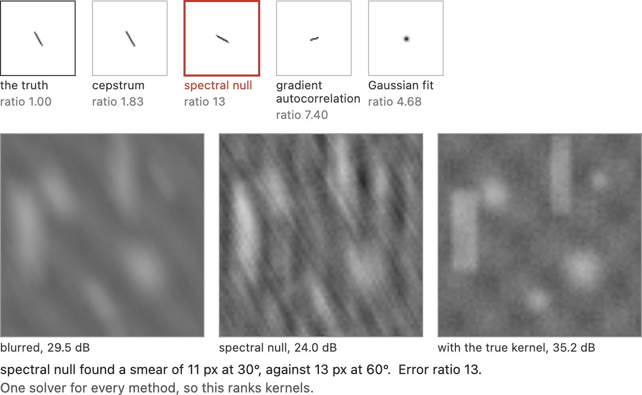
The final deconvolution was not controlled. A blind method estimates a kernel and then runs a non-blind deconvolution with it. If two papers use different non-blind solvers, the comparison measures the solvers as much as the kernel estimates. Hold the non-blind solver and tuning protocol fixed to isolate kernel estimation. Also compare complete pipelines when deployment quality is the question.
Success was judged by appearance. Sharpness is easy to produce and easy to mistake for correctness, and a method that over-sharpens with ringing looks decisive next to one that is faithful and soft.
16.9.2 What to measure⧉
When a kernel is estimated, compare it after resolving allowed normalization, support and shift conventions. Also measure its effect on a fixed reconstruction solver $D$ through
Use the same evaluation crop and parameter-selection policy. This ratio is an image-reconstruction error ratio, not a direct kernel distance. A value near one means similar error under that solver; a near-zero denominator makes it unstable. It can be below one because noise, regularization and kernel mismatch interact.
Report image error and appropriate perceptual comparisons (Chapter 13.12, Measuring a denoiser). Neither metric guarantees a particular visual failure mode. Include edges, text and texture under a common display transform.
Ringing, specifically. Deblurring's signature artifact is oscillation near strong edges, it is not what a global metric penalizes most, and it is what a viewer sees first. Measure it near edges rather than over the frame.
Gradient energy can increase with ringing or noise as well as true detail. Use it as a limited diagnostic, including within a parameter sweep where it can still favor overprocessing. Blinded visual comparison and independent measurements can supply complementary checks.
16.9.3 On what data⧉
Three kinds, and the differences matter more here than in the neighboring parts.
Synthetic blur on sharp photographs gives exact ground truth for both image and kernel, and supports direct kernel tests. Calibrated physical experiments can also provide measured PSFs, with uncertainty. Use both controlled families and measured trajectories to probe the relevant assumptions.
Averaged high-speed frames, as in the GoPro set, give real motion and a target that is itself slightly blurred, and require the dataset's response/averaging variant to be specified (Chapter 16.7, Learned deblurring).
Captured pairs, as in the beam-splitter sets, are real at both ends and carry alignment error and short-exposure noise instead.
A result on one of these says little about the others, and a method that reports on all three is being straightforward with the reader.
16.9.4 What to report⧉
Report the blur model, whether the kernel was known, and the reconstruction method. Hold the non-blind solver fixed when isolating kernel estimation; compare complete pipelines when output quality is the question. Include estimated kernels when available, distortion and perceptual measures, edge crops for ringing, and training and evaluation domains.
Publish intermediate estimates when the method produces them, and report reference preparation, borders, color domain, clipping, training data and cost. Direct image-prediction methods need not return a kernel; their output can still be compared under the same final-image protocol.