14.4 Single-image super-resolution: classical methods⧉
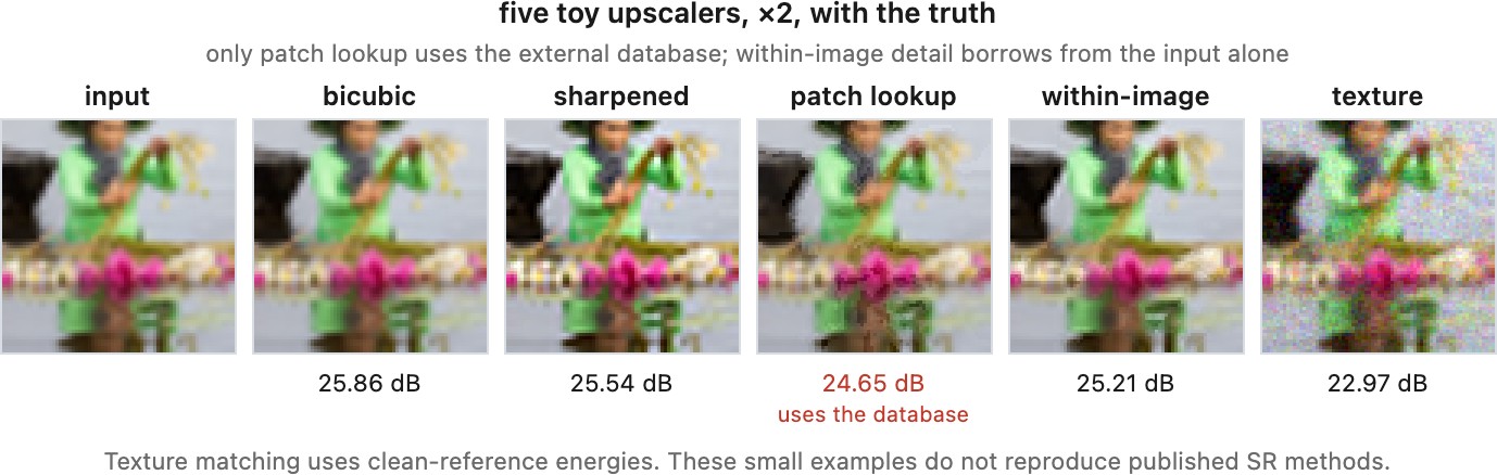
A single photograph can leave several high-resolution images consistent with its samples. Interpolation, patch matching and learned dictionaries select among those possibilities using different assumptions. A sharper result may be more accurate, but sharpness alone does not establish that.
In $y=SBx+n$, a perturbation $v$ with $SBv=0$ changes the fine-grid image without changing its predicted measurement. This null space expresses ambiguity. Near-null directions are also difficult because their effects are small relative to noise.
14.4.1 Interpolation, and what it actually assumes⧉
The baseline is resampling (Chapter 11.1, Warping): evaluate a reconstruction filter on a finer grid. Ideal sinc interpolation exactly reconstructs an ideally band-limited signal from noiseless infinite samples. Bicubic and windowed-sinc filters make practical compromises involving support, ringing and frequency response.
Finite bicubic or Lanczos interpolation does not impose an exact zero spectrum above Nyquist, nor does it generally invert a preceding blur. It produces a smooth continuation of the sampled image under a chosen kernel and boundary convention (Figure 14.1.4).
Compare interpolation with learned reconstruction using the same output size and display sharpening. Error against a reference measures fidelity; visual crispness measures a different property. An interpolation can also ring or alias, so it is not automatically a neutral rendering.
14.4.2 Example-based super-resolution⧉
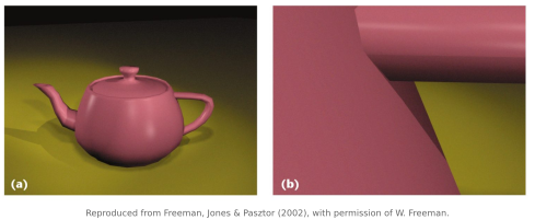
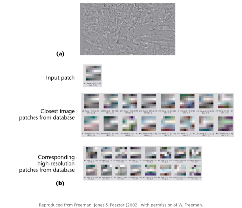
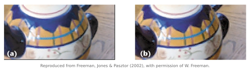
Freeman, Jones and Pasztor's method (Freeman et al. 2002) provides a concrete example of patch-based synthesis. Build a database from real photographs: cut each into small patches, and for every high-resolution patch record the corresponding low-resolution patch. To upscale a new image, cut it into patches, look up each one in the database, and paste in the high-resolution partner.
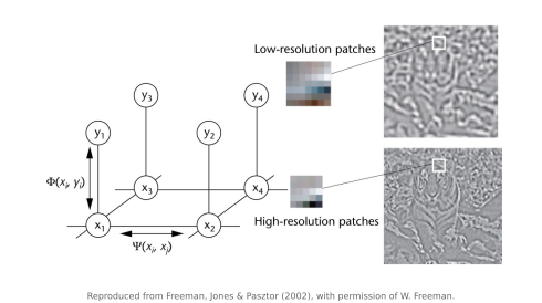
Two details make it work. The lookup uses the patch's high-frequency content after removing its local mean and contrast, to make matches less dependent on local brightness and contrast, with safeguards for nearly flat patches. And neighboring output patches must agree where they overlap, or the result is a mosaic of unrelated fragments, so the selection is posed as a Markov random field over the patch grid and solved with belief propagation. The prior is doing two jobs at once: what a patch should look like, and that neighboring patches should be consistent.
The failure mode is instructive and it is shared by everything after it. The method produces detail typical of its database. A database poorly matched to the subject can supply incorrect texture, especially on text and fine ornament.
14.4.3 Neighbor embedding and the manifold assumption⧉
Chang, Yeung and Xiong (Chang, Yeung & Xiong 2004 (neighbor embedding)) replaced the single nearest neighbor with a combination of several. The assumption is that low-resolution and high-resolution patches lie on corresponding manifolds with the same local geometry, so if a query patch can be written as a weighted combination of its $k$ nearest low-resolution neighbors, the same weights applied to their high-resolution partners give the answer.
Constrain $\sum_jw_j=1$ in the neighbor-embedding fit to reproduce an affine combination of nearby patches. A small ridge penalty can stabilize nearly dependent neighbors. The assumption that these weights also describe the high-resolution partners is learned from the paired data, not guaranteed by the low-resolution fit.
Combining neighbors lets a finite database express more than its individual entries. A query lying between several examples need not copy any one of them exactly. The high-resolution estimate instead follows their local combination. This provides a transition from nearest-neighbor lookup to a fitted mapping, with the limitation that two similar low-resolution patches can still hide very different fine detail.
14.4.4 Sparse coding and dictionary learning⧉
Yang and colleagues (Yang et al. 2010 (sparse representation SR)), and Zeyde and colleagues in a faster form (Zeyde, Elad & Protter 2010), replaced the database with a pair of learned dictionaries. Train a low-resolution dictionary $D_L$ and a high-resolution dictionary $D_H$ jointly on patch pairs, so that a patch and its partner share the same sparse code. Then upscaling has three steps: find the sparse code of the input patch over $D_L$, apply that code to $D_H$, and stitch the results.
# sparse-coding super-resolution, one patch
feat  = high_pass_features(patch_lowres)      # gradients / laplacians, not raw pixels
alpha = solve_lasso(D_L, feat, lam)           # L1-penalized fit, for example with ISTA
patch_hi = D_H @ alpha                        # SAME code, other dictionary
paste_with_overlap_average(out, patch_hi)     # neighboring patches must agree
ISTA Daubechies, Defrise & De Mol 2004 (ISTA) alternates a dictionary-gradient step with soft thresholding. A general dictionary problem does not reduce to thresholding once; orthogonal special cases do. Orthogonal matching pursuit uses greedy atom selection for a different sparsity formulation. SRCNN Dong et al. 2014 (SRCNN) later learned feature extraction, nonlinear mapping and reconstruction jointly, with a useful conceptual connection to this pipeline rather than an exact algebraic equivalence.
A coupled-dictionary method learns low- and high-resolution patch dictionaries whose paired atoms represent corresponding structures. For a new low-resolution patch, find a sparse set of coefficients that explains its features using the low-resolution dictionary. Apply those same coefficients to the high-resolution dictionary, then aggregate overlapping reconstructed patches. Sharing the coefficients is the learned correspondence between resolutions. A coefficient-wise soft threshold is the proximal step for the sparsity penalty; with a general dictionary it is not the entire sparse-coding solve. The repeated gradient-and-threshold iterations explain the connection to unrolled networks while preserving the actual reconstruction procedure.
14.4.5 RAISR: a bank of learned filters, chosen by hashing⧉
RAISR learns a compact bank of local filters and selects among them using image structure. It is a useful example of learning within a small, explicit computational budget.
RAISR (Romano, Isidoro & Milanfar 2016) learns a small bank of linear upsampling filters from low- and high-resolution training pairs. At run time it computes, for each pixel, three cheap statistics of the local gradient, its orientation, its strength and its coherence, quantizes them into a hash, and applies the filter that hash selects. No search, no dictionary, no iteration: a hash and one convolution.
Here $U$ first enlarges the input. The local orientation $\theta$, strength $s$ and coherence $c$ select the filter applied to a patch on that enlarged grid.
The selected filters adapt to local edge statistics. Hash selection makes the overall operator nonlinear even though each selected filter is linear. Negative weights and changes in filter choice can sharpen, ring, or alter small letterforms. This restriction on the architecture limits its behavior but does not certify reconstructed content.
Measure its cost and quality against a particular interpolation implementation; neither runtime nor artifact freedom follows from the method family alone.
RAISR also had a concrete delivery use. In 2017 Google reported using it to reconstruct some Google+ images from smaller transmitted versions, reducing bandwidth for those images (Google's deployment account). The engineering choice was to spend receiver computation on enlargement rather than transmit every displayed pixel. It illustrates how a compact learned filter bank can matter even when it is not the highest-scoring reconstruction model.
14.4.6 The image as its own database⧉
Glasner, Bagon and Irani (Glasner et al. 2009) observed that the patches most likely to match a given patch are elsewhere in the same photograph, at the same scale and at coarser ones. A photograph repeats itself, which is the observation Chapter 13.6, Non-local means and BM3D used to denoise, and it repeats itself across scales too: a small window in a downscaled copy of the image often matches a larger window in the original.
That cross-scale recurrence gives genuine low-to-high pairs from the input alone, with no external database and no training. The prior is the image's own statistics, which is why the method does well on structured scenes, brickwork, windows, text with repeated letterforms, and poorly on unique content.
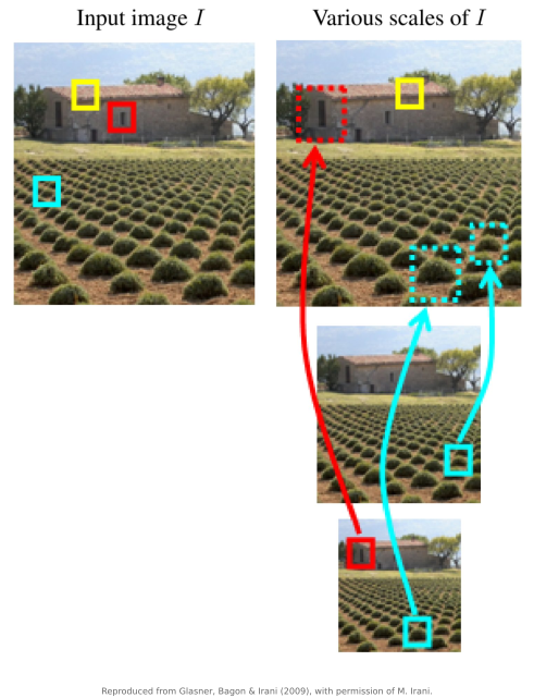
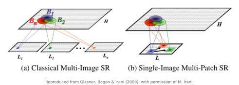
Internal recurrence is useful when comparable patches occur at other scales. It provides examples from the same photograph, but those examples can differ in geometry, shading or material, and they are not independent captures of the target patch.