24.3 Dehazing🔗⧉

A landscape photographed across a few kilometers of hazy air comes back washed out: distant ridgelines fade to a flat, bluish-gray, contrast collapses with distance, and the colors drain away toward the brightness of the sky. The near foreground may look fine while the mountains behind it dissolve into milk. The instinct is to "boost contrast," but a global curve cannot fix it, because the damage is depth-dependent: the far ridge needs far more correction than the near tree, and a single curve has no way to know which pixel is which.

The standard haze model describes contrast loss even with a perfectly focused lens. It neglects spatial blur from multiple scattering, which can matter in dense media. What has happened is scattering: between the scene and the camera, tiny particles (water droplets, dust, aerosols) both attenuate the light traveling from each surface and add their own glow of scattered ambient light (the airlight) and the deeper the scene point, the more of both. So the same inverse-problem template applies again. We will write down the physical image-formation model, notice that it has too many unknowns to invert per pixel, and then watch one statistical observation (the dark-channel prior) provide an estimate of the missing quantity, with recognizable failure cases. The chapter ends one level up, on the tooling that lets us optimize such pipelines at all.

24.3.1 Dehazing as a prior-driven inverse problem🔗⧉

The problem has the same inverse-problem form as the rest of the part. We have an under-determined image-formation model (the archetypal Chapter 7.1, Imaging as Bayesian inference with probabilistic priors) and we add one statistical prior that makes it solvable, exactly the move of blind deblurring in Chapter 16.4, Blind deblurring, even though the physics could not be more different (an unknown convolution kernel in deblurring, atmospheric scattering here). The point is that the same inverse-problem structure appears in both cases.

The physical forward model. Each observed pixel is a blend of two things: the light that actually made it from the scene surface to the camera, dimmed by the haze, plus the haze's own scattered glow. Writing $I$ for the observed (hazy) image, $J$ for the clear scene radiance we want, $A$ for the airlight (the bright, roughly constant atmospheric light, essentially the color of the haze far away), and $t$ for the transmission (the fraction of $J$'s light that survives the trip to the camera, between $0$ and $1$):

Read it back in words: each pixel is the clear radiance attenuated by the transmission, blended with the airlight in proportion to how much was lost. The first term, $J\,t$, is direct attenuation: the scene, faded. The second term, $A(1-t)$, is the airlight: the haze's glow, weighted by exactly the fraction $1-t$ of light that didn't survive. When $t = 1$ (no haze, the near foreground) the pixel is the clear radiance $J$; when $t \to 0$ (deep haze, the far ridge) the pixel washes out entirely to the airlight $A$. Haze is a depth-dependent fade toward $A$. Note the shape: the clear scene enters multiplicatively in the $J\cdot t$ core, radiance times a surviving fraction, the same contrast-is-a-ratio structure L2.6show that recurs across imaging, and it is the airlight term $A(1-t)$, an additive offset, that makes the model affine rather than purely multiplicative, which is exactly why a single global tone curve cannot undo it.

The transmission is not arbitrary: it follows the physics of attenuation through a medium, $t(x) = e^{-\beta d(x)}$, where $d$ is the scene depth and $\beta$ the homogeneous medium's extinction coefficient, including scattering and absorption. This is the same exponential extinction (Beer–Lambert) law that governs any absorbing or scattering medium: light decays multiplicatively with distance. Transmission measures optical thickness. If $\beta$ is known and constant, $d=-\log(t)/\beta$ converts it to distance. Without that calibration, or in spatially varying haze, a transmission map is not a metric depth map.

Underwater imaging also combines direct attenuation and scattered light, but their wavelength dependence is stronger and their effective coefficients need not be equal. Red light usually attenuates faster than blue-green light; the exact behavior depends on the water. Simply assigning one atmospheric transmission to each RGB channel can still be inadequate. Akkaynak and Brown (2026) emphasize a separate practical requirement for quantitative underwater color: retain RAW captures. Camera rendering can irreversibly alter the radiometric relationship before JPEG compression even starts.

Why it is under-determined. Count knowns and unknowns per pixel. We observe $I$: three numbers, the RGB of the hazy pixel. We want to recover $J$ (three numbers), $t$ (one number), and we share a global $A$ across the image. So at every pixel we have three equations and four unknowns (the three components of $J$ plus $t$), before we even fix $A$. The model is hopelessly under-determined as written: infinitely many (clear-scene, transmission) pairs reproduce the same hazy pixel. We cannot invert it from the data alone: we need a prior (Figure 24.3.2⛶ fullscreen).

This is another recurrence of L7.8show: the prior is not optional; see Chapter 14.1, What can super-resolution actually do?. Dehazing is a clear demonstration in the part: the model is literally unsolvable per pixel, and a statistical observation about natural scenes supplies a useful estimate, rather than a uniqueness guarantee.

The dark-channel prior. Here is the observation that breaks the deadlock, due to He, Sun and Tang (2009) and one of the most influential priors in imaging. Take a small nonsky window in a haze-free outdoor photo and look across all three color channels. In almost every such patch, some channel at some pixel is very nearly zero: there is a shadow, a dark or vividly colored surface, a sliver of a deep-saturated object. Pure colorful or shadowed regions are dark in at least one channel; only white or gray, well-lit surfaces are bright in all three, and those are rare in any given small patch of a real outdoor scene. Define the dark channel of an image as the per-patch minimum over both channels and a local window $\Omega(x)$:

The empirical claim (verified on thousands of haze-free outdoor images) is that for many nonsky patches of clear outdoor scenes, $J^{\text{dark}}(x) \approx 0$. Bright white surfaces and sky are important exceptions.

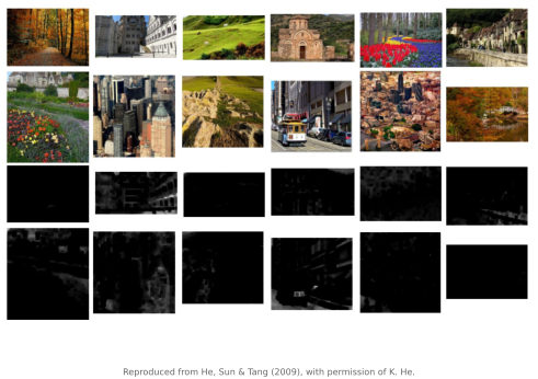
Now watch what haze does to that near-zero dark channel. The airlight term $A(1-t)$ adds a bright, positive amount to every channel, more where the haze is thicker. It lifts the dark channel off the floor. So the dark channel of the hazy image is no longer near zero: its brightness is a direct read-out of how much airlight has been added, which is to say a direct read-out of $1 - t$. How bright the hazy dark channel is $\approx$ how much haze $\approx 1 - t$. Assuming transmission is approximately constant within the window, dividing each channel by its nonzero airlight component and taking the patch minimum gives a clean estimate of the transmission directly from the hazy image:

That statistical regularity supplies the missing unknown (Figure 24.3.2⛶ fullscreen).

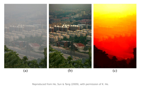
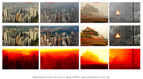
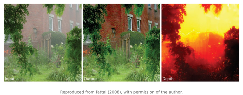
The dark channel was not the first prior to crack this model. A year earlier, Fattal (2008) attacked the same under-determined haze equation with a different statistical assumption (that within a small patch the surface shading and the transmission are locally uncorrelated) and estimated the airlight-independent albedo and the transmission by an independent-component analysis of that local statistic. Different prior, identical skeleton: one regularity about clear scenes supplies the missing unknown.

The pipeline. With the prior in hand, dehazing is four steps:

1. Estimate the airlight $A$. The haziest pixels are the ones whose dark channel is brightest, nearest to pure airlight. So pick the pixels with the highest dark-channel values (the top fraction of a percent), and read $A$ off the brightest of those in the original image. This approximates finding a region dominated by airlight. A bright white object can fool the selection; inspect the estimate rather than assuming the brightest candidate is atmospheric light.
2. Estimate a coarse transmission $\tilde t(x)$ from the dark channel via the formula above. (In practice one keeps a small amount of haze in the far field, a factor like $1-\omega(1-\tilde t)$ with $\omega\!\approx\!0.95$, because a perfectly dehazed distance looks unnaturally flat; some aerial perspective is a depth cue the eye expects.)
3. Refine the transmission's edges. The coarse $\tilde t$ is computed over patches, so it is blocky and its boundaries do not line up with real object edges: it will halo around a sharp silhouette against the sky. The fix is to snap the transmission map to the image's own edges: solve for a refined $t$ that stays close to $\tilde t$ but follows the structure of $I$. He's original paper used soft image matting (a large sparse, edge-aware linear solve, the same matting Laplacian family as colorization in Chapter 10.5, Matting Laplacian); the follow-up guided image filter (He, Sun and Tang, 2010) does the same job far faster, using the hazy image itself as the guide that tells the filter where the edges are. Either way this is an edge-preserving / affinity step, exactly the machinery of Chapter 10.1, Bilateral filtering, reused.
4. Invert the model for $J$. With $A$ and a refined $t$ in hand, solve the haze model pixelwise for the clear radiance: $$ J(x) = \frac{I(x) - A}{\max\!\big(t(x),\,t_0\big)} + A. $$ The clamp $t_0$ (a small floor, $\approx 0.1$) keeps the division well-behaved where transmission is tiny: in the deepest haze almost no signal survived, so dividing by a near-zero $t$ would catastrophically amplify whatever noise is there, the same "inversion amplifies noise" trap that haunted deblurring. The floor caps that amplification, accepting a little residual haze in the far distance rather than a face full of noise.

Dehazing needs both a transmission estimate and an airlight estimate. The dark-channel prior gives a useful starting point in many outdoor scenes, but white surfaces, sky, nonuniform airlight, and depth boundaries can violate it. The transmission floor trades residual haze against amplified noise; clipping and quantization are not reversible. Learned methods replace or supplement these assumptions with training-data statistics (Chapter 7.3, Deep learning), and video de-weathering can also exploit temporal evidence (Missing stuff, bugs#De-weathering (fog, rain)).

24.3.2 Differentiable image pipelines and algorithm optimization (Halide)🔗⧉

Step back and look at everything the last several chapters built. Deblurring, super-resolution, colorization, dehazing: every one is an optimization with a prior, a pipeline of operations (take gradients, estimate a map, refine with an edge-aware filter, invert a model) with knobs at every stage: filter weights, the patch size $\Omega$, the airlight percentile, the floor $t_0$, the regularization strength. Who optimizes the pipeline itself? When a restoration or full camera ISP has dozens of such parameters (or whole stages you'd like to learn) you want to tune them by gradient descent against a quality loss, the way we train anything else. For that, two things have to be true of the pipeline: it must be fast (you'll run it thousands of times), and gradients must exist or be approximated for the parameters being optimized. Discrete choices such as integer patch size and schedule structure require a separate search. Hard minima are piecewise differentiable; clipping can make gradients vanish, and percentile selection needs particular care.

Halide. Ragan-Kelley et al. (2013) is a language built on one decisive separation: it splits what an image pipeline computes (the algorithm, the math) from how it runs (the schedule, meaning the tiling, vectorization, parallelism, and fusion of stages across the memory hierarchy). You write the algorithm once, in clean mathematical form, and then separately describe a schedule; the compiler combines them. One algorithm admits many schedules, so schedules can be tuned for CPU and GPU execution without rewriting the mathematical algorithm. Performance still depends on the schedule and hardware. This decoupling is why Halide became the substrate a great deal of production computational photography is actually implemented in: the burst pipelines, the local tone operators, the filters of this very part.

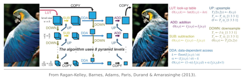
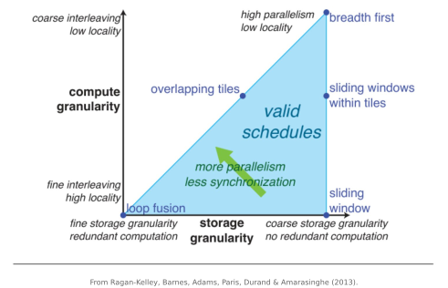
Differentiable Halide. Li et al. (2018) add automatic differentiation through a Halide pipeline. Once you can backpropagate through the whole sequence of stages, two doors open at once. You can tune the pipeline's parameters by gradient descent: pose "find the dehazing/deblurring/ISP settings that minimize a quality loss on a dataset" as plain optimization through a fast, scheduled pipeline. And you can drop a classical pipeline in as a layer inside a neural network, so hand-built physics and learned components train end to end together. "Learn the filter" and "tune the algorithm" become the same gradient-descent loop.

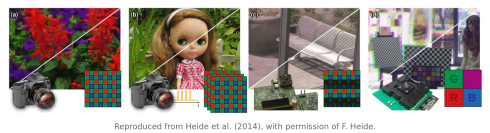
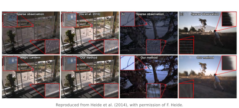
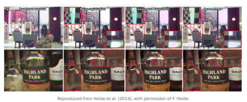
FlexISP (Heide et al., 2014) illustrates the related idea of expressing an ISP as a joint inverse problem with image priors. Its iterative optimization is not the same claim as automatic differentiation through an ISP for parameter learning. One optimizes an image; the other can differentiate a training loss through the operations that produce it. Both benefit from efficient implementations, and both can combine physical models with learned components. See Part 29, Making computational photography code fast for the implementation ideas, including code generation and the separation between an algorithm and its execution schedule.