10.9 Seam optimization⧉
You have stitched a panorama and one seam will not go away. Two photographs overlap, already aligned so the static background registers, and somewhere in that overlap you must decide, pixel by pixel, which photograph to keep. Wherever the decision flips from one source to the other, there is a seam. Run it straight down the middle and a hard line appears. The two exposures never matched perfectly, a cloud drifted between frames, a pedestrian walked through. Hide the line by feathering across the boundary and you swap the line for ghosting: the pedestrian, half from each frame, becomes a transparent double. The hard cut and the soft blend both fail, and for the same reason: they put the seam in the wrong place.
The fix is to choose where the seam goes: route it through the hedge, the gravel, or the cluttered roofline (anywhere the two photographs already agree, or the texture is so busy that a switch cannot be seen), and keep it out of the flat sky and the blank wall, where the smallest mismatch would shout. That, stated once, is the entire subject of this chapter: find the least-noticeable cut. It is the precise dual of the edge-preserving filtering we just finished. Filtering uses boundaries to limit mixing; seam selection uses image structure to decide where a change of source or a removal will be least objectionable.
These tasks use related graph machinery but different costs. Live-wire selection follows an object edge; seam carving usually avoids deleting one; compositing prefers locations where switching sources is unobtrusive. There is no universal rule to cut through texture or avoid smooth regions.
What unifies the methods is one idea wearing three hats. Lay the image out as a graph (or a grid, which is just a graph with a regular neighborhood), attach a cost to cutting at each place, and ask an optimizer for the cheapest cut. When the cut is a one-dimensional path running top to bottom, the optimizer is dynamic programming. When the cut is a two-dimensional boundary separating one region from another, the optimizer is min-cut / max-flow on the graph. When we want a balanced split with no seeds at all, the optimizer is a spectral relaxation (normalized cuts). Between methods the optimizer rarely changes; you take it off the shelf. What changes is the energy: what you decide to penalize. That is the lesson this chapter exists to teach.
Many image edits are discrete optimization on a graph or grid, whether dynamic programming (a least-cost path), min-cut / max-flow (a globally optimal boundary), or a spectral relaxation (normalized cuts), and the energy (affinity) you choose is the whole design. The optimizer is generic and off the shelf; what you penalize (gradient magnitude along a seam, label disagreement across an edge, the cost of severing two regions) is the entire design. Read this as the L10.1 affinity principle from Chapter 10.1, Bilateral filtering turned inside out. There, the affinity between two pixels said "average these together." Here, the very same quantity, sitting on a graph edge, says "do not cut here." High affinity (similar neighbors) marks an expensive place to cut; low affinity (a genuine edge) marks a cheap one. Design that cost well and a generic min-cut often returns a boundary close to the one a person would have drawn; when it does not, the fix is usually in the energy, not in the optimizer. (Registered as new lesson L10.5 · image edits as discrete optimization on a graph (the energy is the design), first appearance here. Extends L10.1. Also relevant downstream: graph-cut photomontage composed with a Poisson blend; compositing / segmentation / matting; texture synthesis; stereo and Markov-random-field labeling.)
10.9.1 Find the non-edges: least-noticeable cuts⧉
For a composite, source agreement and geometric continuity matter. A smooth sky can be a good seam location when both images agree; a busy hedge can be poor when it moves between exposures. Choose a cost that measures the relevant mismatch and inspect the resulting join.
The panorama makes the recipe concrete and resolves the earlier forward-reference from the panorama alignment-and-blending chapter: RANSAC (random sample consensus) Fischler & Bolles 1981 for the alignment, then the blend; → Chapter 20.2, Automatic panorama stitching from multiple views and feature matching, which promised that "the optimal boundary between two images" would be found by graph cut. Build a difference map over the overlap (a per-pixel record of where bad things happen): where the two aligned images disagree in color, where a moving object shows up in one frame but not the other. Then find the boundary that crosses the fewest of those bad pixels. A seam that threads around every disagreement leaves a join nobody can see. The blending chapter's hard line and ghosted soft line were both just the price of not choosing the boundary.
Two regimes follow, and the chapter is organized around them. In the interactive regime, a person guides the cut and the algorithm snaps it to the nearest good path: intelligent scissors and snakes, the historical ancestors. In the automatic regime a global optimizer finds the whole cut unaided: seam carving, graph cut, normalized cuts, the main line. We meet the ancestors first because they make "the cut is a least-cost path" tangible with a human in the loop; the automatic methods are then the same idea with the human removed.
10.9.2 Intelligent scissors / live-wire: the cut as a least-cost path⧉
The first tool to make the principle interactive is intelligent scissors, also called live-wire (Mortensen & Barrett 1995). It is a selection tool. You want to trace an object's outline to cut it out, and tracing it freehand, pixel by pixel, is slow and shaky. Intelligent scissors lets you click one seed point on the boundary; then, as you sweep the cursor roughly along the object's edge, a "live wire" snaps to the strongest nearby edge and traces the boundary for you in real time. When the path looks right, click to anchor it and carry on. The tool does the precise edge-following; you supply only the rough intent (Figure 10.9.1).
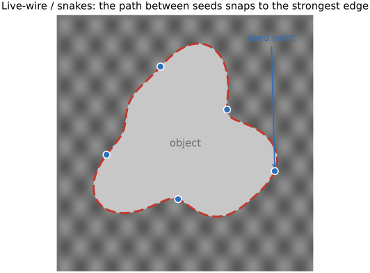
The mechanism is a shortest path on a cost graph, and it is the cleanest first instance of this chapter's machinery. Make every pixel a node, connect neighbors, and set each connection's cost low where the image gradient is high. A good boundary runs along strong edges, so we want the cheap path to be the one that hugs them. The cost is the inverse edge magnitude, plus terms that reward following the edge tangent, perpendicular to the image gradient, smoothly rather than cutting across it. Now run Dijkstra's algorithm from the seed: it returns the least-cost path from the seed to every other pixel at once, so the optimal wire to the cursor's current position is already computed and can be drawn instantly as the cursor moves. Drift the cursor over a smooth region and the cheapest path still detours to ride the nearby edge. That is the "snap to the boundary" behavior you feel.
The main pattern of the chapter is already visible in this first example: this is the same machinery we will use for seam carving (a least-cost path on a gradient-derived energy) aimed at the opposite goal. Live-wire makes its cost low along edges, so the path follows an edge to select it. Seam carving will make its cost low in flat regions, so the path avoids edges and threads through non-content. The optimizer (a least-cost path) is identical; only the energy, and so the meaning of the cut, differs. The energy is the design.
10.9.3 Snakes (active contours): the continuous cousin⧉
A snake, or active contour (Kass, Witkin & Terzopoulos 1988), is the continuous, variational counterpart of live-wire. In place of a discrete path on a pixel graph, a snake is a smooth curve $v(s)$ (picture an elastic loop dropped near an object) that relaxes onto the object's boundary by minimizing an energy. Where live-wire is combinatorial, the snake is calculus: it flows downhill on an energy functional until it settles into the boundary, like a deformable band shrink-wrapping the object.
The energy has three parts, and reading them back in words is the whole intuition:
The internal term keeps the curve well-behaved (smooth, and not too crinkly) through two penalties on the curve's own shape,
where $\alpha$ is an elastic tension (penalizing length, so the curve wants to be short and not stretch) and $\beta$ a bending stiffness (penalizing curvature, so the curve wants to be smooth and not kink). The image term pulls the curve toward strong edges,
negative because we minimize energy, so the curve is drawn to places where gradient magnitude is large: the boundaries. The constraint term $E_\text{con}$ lets a user nudge the curve, pinning a point or pushing it off a bad local fit. Together: be smooth (internal), sit on the edges (image), obey my hints (constraint). Minimizing $E$ is gradient descent, which in discretized form is a sparse banded linear solve at each step, the same linear-algebra machinery as Chapter 6.7, Image formation as a linear system, now driving a curve instead of an image.
The limitation is that a snake is local. It descends to the nearest energy minimum, so it needs a decent initialization and can lodge on a spurious edge or fail to crawl into a deep concavity. That fragility is exactly what motivates the global optimizers next: methods that find the best boundary outright, with no initialization and no local minima to trap them. The many patches for snakes (balloon forces that inflate the curve, gradient vector flow that broadens an edge's pull, level-set reformulations that let the curve change topology) we note only in passing; the global graph cut is the cleaner answer.
10.9.4 Graph cut: globally optimal boundaries by min-cut / max-flow⧉
The leap from local to global is the heart of the chapter (Boykov & Jolly 2001). Stop tracing a curve and instead pose the cut as a binary labeling: every pixel is assigned a label (object or background) and the boundary is wherever the labels change. Choosing the labels well is a single optimization whose minimum, in the binary case, is found exactly and globally by min-cut / max-flow on a graph. There is no initialization and no local-minimum trap. In the binary submodular case, this gives the global optimum.
For binary labels, each pairwise term must satisfy $V_{pq}(0,0)+V_{pq}(1,1)\leq V_{pq}(0,1)+V_{pq}(1,0)$ for the standard graph-cut construction. Nonnegative Potts disagreement penalties satisfy this condition. A min-cut is globally optimal for the specified representable energy with fixed parameters; it does not guarantee the intended object boundary or the optimum of a larger alternating estimation procedure.
The energy is the same shape that runs through all of computer vision:
Read it back in two pieces. The data term $D_p(L_p)$ says how well pixel $p$ fits each label on its own, built from user scribbles ("these pixels are object, those background") turned into color models, so $D_p$ is small when $p$'s color matches the label it is handed. The smoothness term $V_{pq}(L_p, L_q)$ is a penalty paid whenever two neighbors $p$ and $q$ receive different labels: it is what makes the boundary short and coherent instead of a speckled mess. The design choice is to make $V_{pq}$ small across true edges, i.e. small wherever the colors of $p$ and $q$ already differ a lot. Then the boundary, which must break some neighbor pairs, prefers to break the pairs that already differ: it prefers to cut along edges. That is the panorama principle, now written as an energy.
The smoothness weight $V_{pq}$ is not a new idea: it is the L10.1 affinity from Chapter 10.1, Bilateral filtering, read as a cost of cutting. There, the affinity (large when $I_p \approx I_q$) said "these two pixels belong together, average them." Here, the same quantity says "these two pixels belong together, so it is expensive to put a boundary between them." Make $V_{pq}$ large for similar neighbors (do not cut here, they match) and small for dissimilar ones (cheap to cut, there is already an edge), typically $V_{pq} \propto \exp(-\lVert I_p - I_q\rVert^2 / 2\sigma^2)$, the bilateral range weight exactly. It is also the very same object as the colorization affinity and the matting Laplacian Levin, Lischinski & Weiss 2008 (closed-form matting). One similarity measure, used to connect in the filtering chapter and to separate here.
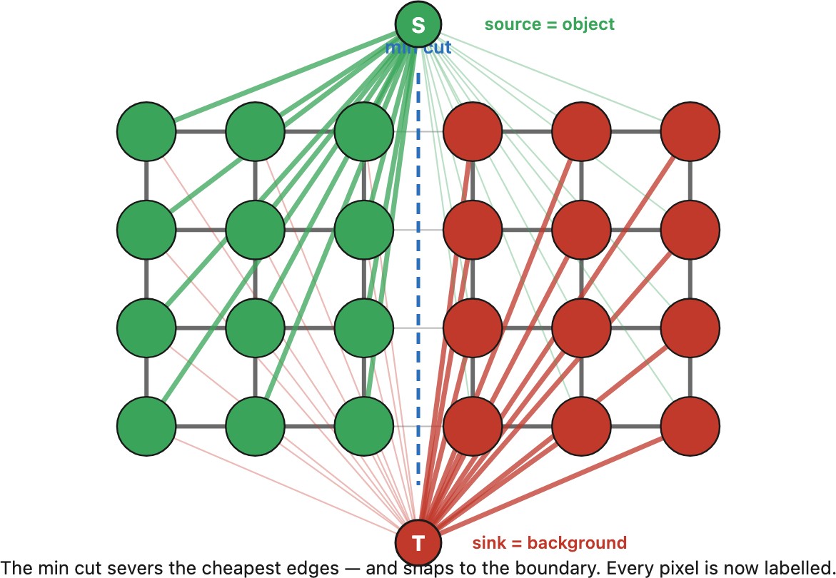
The graph construction makes "min-cut" literal (Figure 10.9.2). Every pixel is a node; add two extra terminal nodes, a source standing for object and a sink standing for background. Connect each pixel to both terminals with t-links whose weights are the data costs $D_p$: a pixel that strongly looks like object gets a fat link to the source and a thin one to the sink. Connect neighboring pixels with n-links whose weights are the smoothness costs $V_{pq}$. Now a cut that severs the graph into a source side and a sink side, dropping every pixel onto one terminal, is a labeling, and the total weight of the severed edges is exactly the energy $E(L)$. So the minimum-energy labeling is the minimum-weight cut, and by the max-flow / min-cut theorem that cut is found by pushing maximum flow from source to sink (Boykov & Kolmogorov 2004 give a max-flow algorithm tuned for these grid graphs). The min cut slices through the cheap edges (the ones across real image edges, where $V_{pq}$ is small) and returns the object boundary.
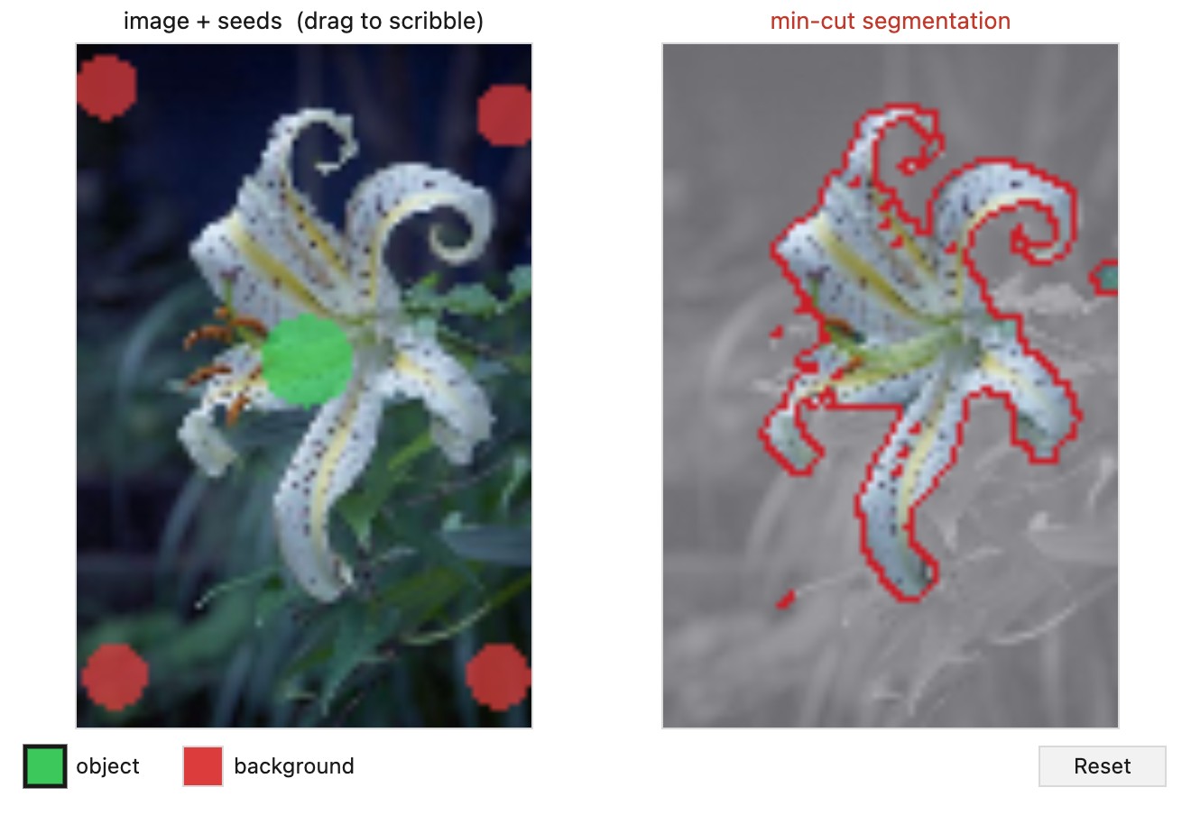
The construction is easier believed when you can drive it (Figure 10.9.3). Scribble a few object and background seeds on a real photo and a max-flow solver returns the exact minimum cut: the boundary snaps to the object, threading the cheap n-links along its edges. The smoothness weight $\lambda$ is the one knob that matters: too small and the cut chases color noise into a ragged boundary; too large and it ignores the object entirely to buy a short, smooth cut.
A named but undeveloped extension is multi-label optimization. With more than two labels (photomontage choosing among several source photos, stereo choosing among many depths, denoising choosing among many intensities) the exact problem is NP-hard. It is solved approximately, and very well, by $\alpha$-expansion (Boykov, Veksler & Zabih 2001): iterate a sequence of binary graph cuts, each asking "which pixels should switch to label $\alpha$?", cycling through the labels until nothing improves. The other famous extension (GrabCut, which makes the cut effortless to drive) earns its own section next.
10.9.5 GrabCut: interactive cutout from a single rectangle⧉
Plain graph cut still asks the user for two things: object scribbles and background scribbles, enough of each to fit the color models that feed the data term $D_p$. GrabCut (Rother, Kolmogorov & Blake 2004) removes almost all of that work, and in doing so became the background-removal tool that shipped for years inside Microsoft Office. The user drags one loose rectangle around the object. Everything outside is declared background (a hard constraint that never changes); everything inside is unknown, and that is the entire interaction.
The trick is to treat the color models as unknown parameters estimated jointly with the segmentation. GrabCut replaces the fixed color models with two Gaussian mixture models (GMMs) in RGB (one for foreground, one for background, five components each) and writes the same Gibbs energy as before, $E = U(\alpha,\mathbf{k},\theta) + V(\alpha)$. The data term $U$ is the negative log-likelihood of each pixel's color under the GMM component of its assigned label (small when the model explains the color well); the smoothness term is the familiar contrast-sensitive Potts penalty $V = \gamma\sum_{(m,n)}[\alpha_m\neq\alpha_n]\,e^{-\beta\lVert z_m - z_n\rVert^2}$ (the L10.1 affinity again), cheap to cut across real edges, with $\beta$ set automatically from the image's mean squared neighbor contrast so it self-adapts to high- and low-contrast scenes.
Because the GMM parameters $\theta$ are unknown, GrabCut iterates: this is the "iterated graph cuts" of its title. Each round does three things, holding the others fixed: (1) assign every pixel to the best-fitting component of its current label's GMM; (2) re-learn each GMM's weights, means, and covariances from the pixels currently wearing that label; (3) re-segment with a single global min-cut, the binary graph construction above. Every step lowers the same energy, so the loop is monotone and converges in a handful of rounds. The picture to keep is a virtuous cycle: the foreground model is initialized from a contaminated set (the whole rectangle interior, mostly object but with background in the corners) and as the cut peels those background-colored pixels away, the model purifies, which sharpens the next cut, which purifies the model further.
Two finishing touches complete it. A border-matting step estimates a soft alpha in a narrow band straddling the boundary, replacing the one-pixel-jagged silhouette with an anti-aliased edge fit for compositing, a lightweight precursor to the matting Laplacian gestured at above. And the user keeps a veto: optional foreground / background touch-up strokes impose hard constraints exactly like Boykov–Jolly's scribbles, but now as cheap cleanup on an already-good result rather than required input.
GrabCut is, in the end, a color-distribution method, and its failures all follow from that. When foreground and background share colors (camouflage, a gray cat on gray gravel) the two GMMs overlap, the data term goes blind, and the result collapses onto whatever the smoothness term prefers; wispy structure (hair, smoke) defeats the hard cut and only partly survives border matting. These are exactly the cases where today's learned matting networks and promptable models like SAM (Segment Anything) (Kirillov et al. 2023) have taken over, trading hand-built color GMMs for learned semantic features. But GrabCut remains the canonical classical energy formulation, and the clean bridge from the graph-cut machinery of this chapter to the matting it feeds, which is why the machinery lives here while the matting application is cross-referred to Part 19, Layers, transparency, compositing, and matting.
10.9.6 Normalized cuts: the spectral relaxation⧉
Plain min-cut has a bias worth confronting head-on. If you minimize the raw weight of a cut with no terminals and no seeds (just "split this image into two pieces as cheaply as possible") the cheapest split is almost always to lop off a single isolated pixel (or a tiny corner), because severing one weakly-connected node cuts very little weight. Min-cut is biased toward tiny, unbalanced cuts. When we actually want a balanced partition (roughly object-sized against roughly background-sized) raw cut weight is the wrong objective.
The fix is normalized cuts (Shi & Malik 2000): divide the cut weight by how strongly each side is connected to the whole, so a split that strands a tiny fragment is penalized for that fragment's feeble total connection. With an affinity weight $w_{uv}$ on every pair of nodes (again the L10.1 affinity, color and spatial similarity), set $\mathrm{cut}(A,B) = \sum_{u\in A,\, v\in B} w_{uv}$ and the association $\mathrm{assoc}(A,V) = \sum_{u\in A,\, t\in V} w_{ut}$ (how strongly side $A$ connects to everything), and minimize
The normalization discourages separating a weakly associated fragment solely because its raw cut is small. It balances association, not necessarily pixel counts, and does not make the objective diverge for every small region. Same affinity input as graph cut; a different, balance-aware objective.
How it is solved we keep to intuition; the eigenvector machinery is deferred to the appendix. Exact normalized cut (Ncut) is NP-hard, but a relaxation is available: allowing the binary "which side" indicator to take continuous values turns it into a generalized eigenproblem
where $W$ is the affinity matrix and $D$ its diagonal degree matrix (each node's total affinity). (For the eigenvector / spectral background this leans on, namely eigenvalues, eigenvectors, and the generalized problem, see Chapter 45.2, Refreshers → linear algebra; we use the result here, not the derivation.) The second-smallest eigenvector of this system is a smooth, real-valued "soft partition" of the image; threshold it for the two regions, and recurse for more. Without the linear algebra, the point is this: there is a spectral route to the best boundary, an eigenvector computation, running alongside the combinatorial route of graph cut. Binary graph cut is combinatorial and exact for a representable fixed energy; its data terms can come from seeds or other evidence. Normalized cut uses a spectral relaxation of a different objective and does not need foreground seeds. Two answers to the same question (where is the best boundary?) fed by the same affinity.
10.9.7 Seam carving: content-aware resize by DP⧉
Now the automatic method that gives the chapter its name (Avidan & Shamir 2007). The problem is content-aware resizing (or retargeting): a wide photo has to fit a tall phone screen, or a square thumbnail, and the two obvious options are both poor. Uniform scaling squashes every face; cropping throws away the edges of the scene. Seam carving does neither. It changes the aspect ratio by removing the least-important pixels, one connected seam at a time, so salient content keeps its shape while the boring regions quietly shrink (Figure 10.9.4).
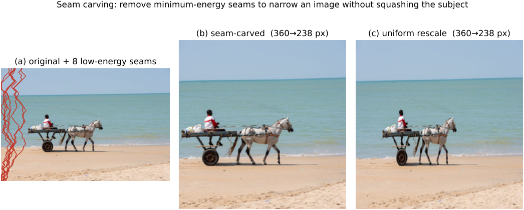
Carve it yourself (Figure 10.9.5): drag the width down and watch the DP remove one minimum-energy seam at a time, the removed seams piling up in the flat sky and water while the skyline holds its shape.
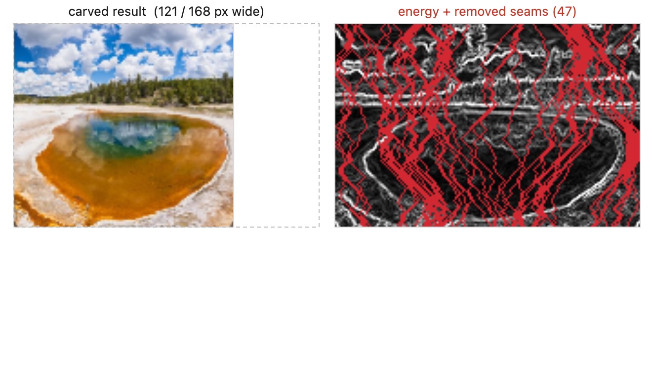
A seam is the unit of removal: an 8-connected, top-to-bottom path with exactly one pixel per row, where each row's pixel lands within one column of the row above (so deleting it leaves a coherent image one pixel narrower). Among all such paths we want the one of minimum total energy, where the per-pixel energy is gradient magnitude, a proxy for importance or saliency:
The cheapest seam threads through low-energy, low-detail regions (flat sky, blurred background, smooth wall) and avoids the subject, whose edges are expensive to cross. Remove it and the photo narrows by one pixel where it could least be missed. Recompute costs after removal. For enlargement, find several seams on a temporary reduced image and map them back before insertion; repeatedly duplicating one seam can stretch an obvious stripe.
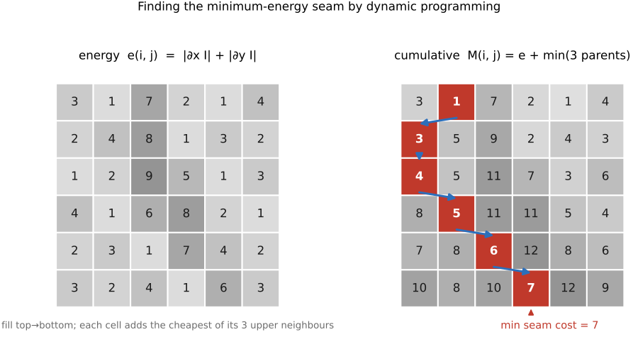
The mechanism is the same least-cost path as live-wire, now solved by dynamic programming, and Figure 10.9.6 walks the table. Build a cumulative-energy table $M$ top-down. The first row is just the energy. For every later row, the cheapest way to reach pixel $(i,j)$ is its own energy plus the cheapest of the three pixels it could have descended from:
Read it back: "the cheapest way down to me is my own cost, plus the cheapest way down to my best parent." When the table is full, the bottom row holds the total cost of the best seam ending at each column; take $\arg\min_j M(H-1, j)$ with zero-based rows for the cheapest endpoint, then back-trace upward (at each step step to whichever of the three parents supplied the minimum) to recover the seam itself. One pass down to fill $M$, one pass up to read off the path:
M[0, :] = e[0, :]
for each row i from 1 to H-1:
    for each column j:
        valid = {k in {j-1, j, j+1} such that 0 <= k < width}
        parent[i,j] = argmin over k in valid of M[i-1,k]
        M[i, j] = e[i, j] + M[i-1,parent[i,j]]

j = argmin over columns of M[H-1, :]
seam = [(H-1, j)]
for each row i from H-1 down to 1:
    j = parent[i,j]
    seam.prepend((i-1, j))
return seam
Seam carving uses a directed acyclic graph, so a row-ordered dynamic program suffices. Live-wire permits more general image paths and uses a shortest-path algorithm such as Dijkstra. Removing the best seam is exact for the current cost image; repeatedly doing so is greedy and need not give the best final resized image.
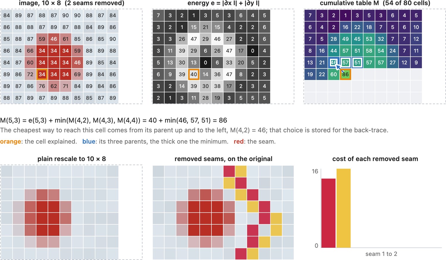
To watch the table fill, run the same program on an image a dozen pixels wide (Figure 10.9.7): each step shows the three parents a cell compares and the one it keeps, and the back-trace follows those stored choices up from the cheapest cell of the last row.
The same program at the size of a real picture, with nothing on screen but the result (Figure 10.9.8), shows what the method is for and where it breaks.
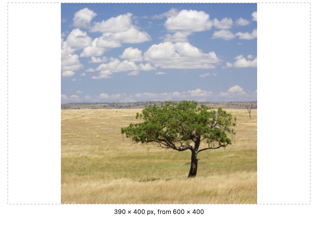
The limit is well known. Seam carving fails on busy or structured images. If there is no low-energy path, as in a packed crowd, a brick wall, or a face filling the frame, every seam must cross something, and carving puts kinks in straight lines and dents in faces. Better energies help: forward-energy scores the new edges a removal would create rather than the ones it removes, and saliency maps or face detectors can be folded into $e$ to protect what matters. But seam carving is a tool for images with slack in them, not a universal resizer.
10.9.8 Time-lapse via DP: a seam through time⧉
The same least-cost-path idea applies when the axis is time rather than space. Assembling a smooth time-lapse (a day-to-night sequence, a season's worth of one tree) out of a pile of candidate frames or exposures is the same dynamic program, with time as the running axis. Lay the candidate frames in a column per time step; cost a transition from one frame to the next by the discontinuity it introduces (an exposure jump, a color shift, a lighting flicker); and run a DP to pick the one frame per step that minimizes the total jump across the whole sequence. It is the seam recurrence with frames for pixels and time for rows.
No dedicated slide or transcript was found for the time-lapse-via-DP example; this section is written from the outline and standard practice as a short bridge between seam carving and video textures. Treat its scope as provisional: it may be trimmed to a single sentence under seam carving, or expanded if a source surfaces.
10.9.9 Video textures: looping a seam in time⧉
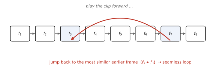
The same time-axis cut becomes a product: video textures (Schödl et al. 2000) turn a short clip of a stochastic, repetitive phenomenon (a flame, a fountain, a waving flag) into an arbitrarily long, seamless loop that never visibly repeats, by finding good transitions (pairs of frames similar enough that playback can jump between them without the eye catching the cut) and folding the clip back on itself there (Figure 10.9.9). It is exactly the seam idea applied to time. The full method (the frame-distance matrix, the dynamic-programming cost propagation, the audio analog, and a live demo) is developed in its own home in the video part, Chapter 30.8, Video textures.
10.9.10 GraphCut textures & photomontage: cut, then blend⧉
Two applications close the chapter by showing the seam machinery composing with the rest of the part.
GraphCut textures (Kwatra et al. 2003) is graph cut aimed at texture synthesis. To extend a texture, or composite two overlapping images, place the pieces so they overlap and run a min-cut through the overlap region to choose the seam: the boundary that picks, pixel by pixel, the path where the two sources agree best (smoothness cost small where the patches match). The min cut routes the join through the places the two textures are indistinguishable, so the synthesized texture has no visible patch boundaries. It is the texture-synthesis sibling of panorama seam-finding: the same "cut where the sources agree" idea, now tiling a plane with texture instead of stitching two photos.
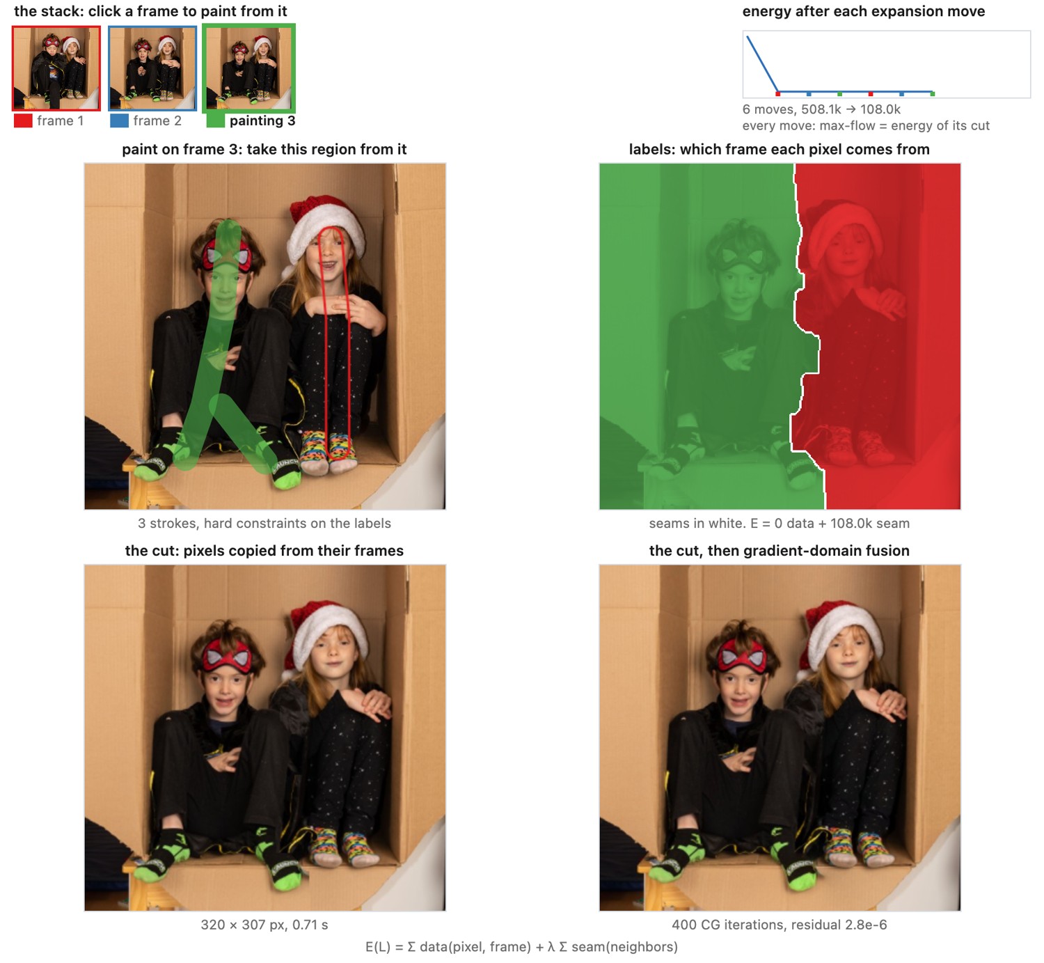
Interactive digital photomontage (Agarwala et al. 2004) is the clean statement of how the three legs of EDGES MATTER compose, and it is shared with Chapter 10.8, Poisson image editing for exactly that reason. The pipeline is cut, then blend. First a graph cut chooses which source photograph contributes each pixel. The user paints rough strokes ("take the eyes from this frame, the smile from that one") and a multi-label graph cut finds seams between sources that fall along edges where switching is cheap. That settles where to switch. Then a gradient-domain (Poisson) blend reconstructs across those seams, absorbing any residual exposure or color mismatch the cut could not avoid. That handles hiding what is left. So the seam picks the boundary (this chapter) and Poisson hides the leftover step (Chapter 10.8, Poisson image editing): cut along the edges, then reconstruct across the seam. It is the tidiest example in the book of two EDGES-MATTER methods working as a single tool, and the explicit reason the two chapters cross-refer.
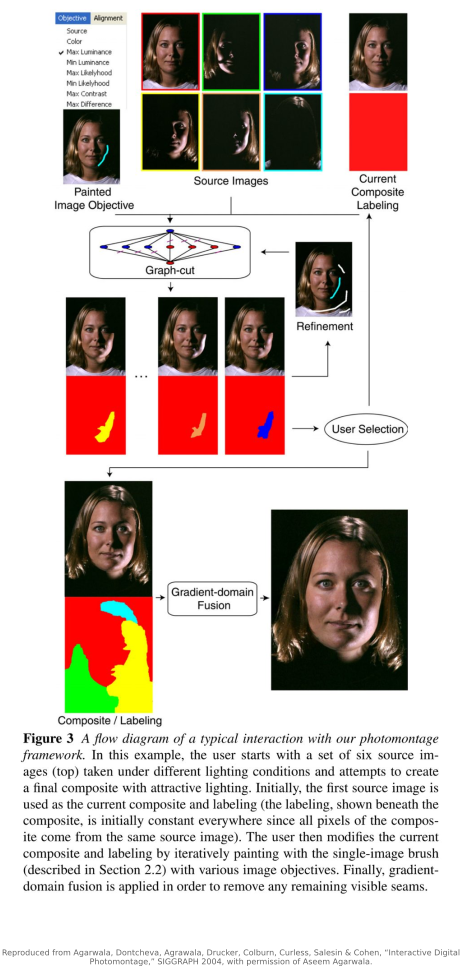
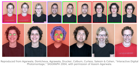
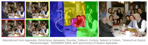
You can run the whole pipeline on three stacks or on your own frames (Figure 10.9.13). The multi-label cut is minimized by alpha-expansion (Boykov et al. 2001): for each frame in turn, every pixel either keeps its label or switches to that frame, and the best such move is one exact minimum cut. On the exposure bracket the cut alone leaves a brightness step along every seam, and the fusion removes it. On the group shots the frames already agree in brightness, and the work is all in where the seams go.
10.9.11 Where this connects: MRFs and beyond⧉
The graph-cut energy
, a per-pixel data term plus a pairwise smoothness term, is a pairwise Markov random field (MRF): a prior that says "labels should agree with the evidence ($D_p$) and with their neighbors ($V_{pq}$)." Graph cut and belief propagation are two ways to do inference in that MRF, i.e. to find the most probable labeling. The same template governs stereo (label = disparity), denoising (label = clean intensity), and optical flow (label = motion). The fuller Bayesian / MRF treatment lives with Chapter 6.7, Image formation as a linear system and segmentation, cross-referred rather than developed here.
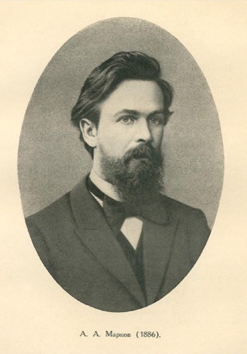 Andrey Markov (1856–1922) studied chains of events in which the next state depends only on the current one, not on the whole past: the Markov property. Lift that from a chain to a grid and you get the Markov random field above: given its neighbors, a pixel's label is independent of the rest of the image. The data-plus-pairwise energy that graph cut and belief propagation minimize is the simplest such model, with interactions only between pairs of neighbors; richer MRFs have larger cliques. The same local-dependence assumption powers patch-based texture synthesis, stereo, and labeling. He first demonstrated his chains by tallying the runs of vowels and consonants in Pushkin's Eugene Onegin. Portrait: before 1922, public domain (via Wikimedia Commons).
Recap: big lessons of this chapter
Many image edits are discrete optimization on a graph or grid, whether dynamic programming (a least-cost path), min-cut / max-flow (a globally optimal boundary), or a spectral relaxation (normalized cuts), and the energy (affinity) you choose is the whole design. The optimizer is generic and off the shelf; what you penalize (gradient magnitude along a seam, label disagreement across an edge, the cost of severing two regions) is the entire design. Read this as the L10.1 affinity principle from Chapter 10.1, Bilateral filtering turned inside out. There, the affinity between two pixels said "average these together." Here, the very same quantity, sitting on a graph edge, says "do not cut here." High affinity (similar neighbors) marks an expensive place to cut; low affinity (a genuine edge) marks a cheap one. Design that cost well and a generic min-cut often returns a boundary close to the one a person would have drawn; when it does not, the fix is usually in the energy, not in the optimizer. (Registered as new lesson L10.5 · image edits as discrete optimization on a graph (the energy is the design), first appearance here. Extends L10.1. Also relevant downstream: graph-cut photomontage composed with a Poisson blend; compositing / segmentation / matting; texture synthesis; stereo and Markov-random-field labeling.)