19.2 Segmentation⧉
A selection lets an editor brighten a face or replace a sky without affecting the rest of the image. A binary segmentation labels pixels by region; some tools also produce soft confidence scores. Neither alone recovers the mixed foreground and background colors at a strand of hair.
19.2.1 Segmentation: cutting the object out⧉
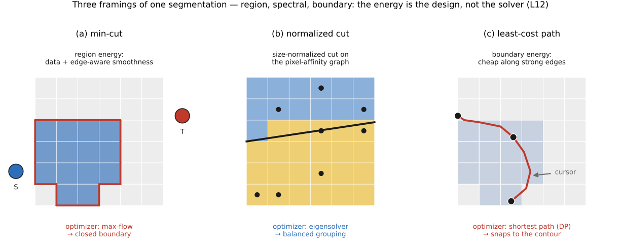
Graph cuts, normalized cuts and intelligent scissors use different graph objectives. A global optimum of one objective need not be the desired object boundary; model design and user constraints determine what the optimizer prefers.
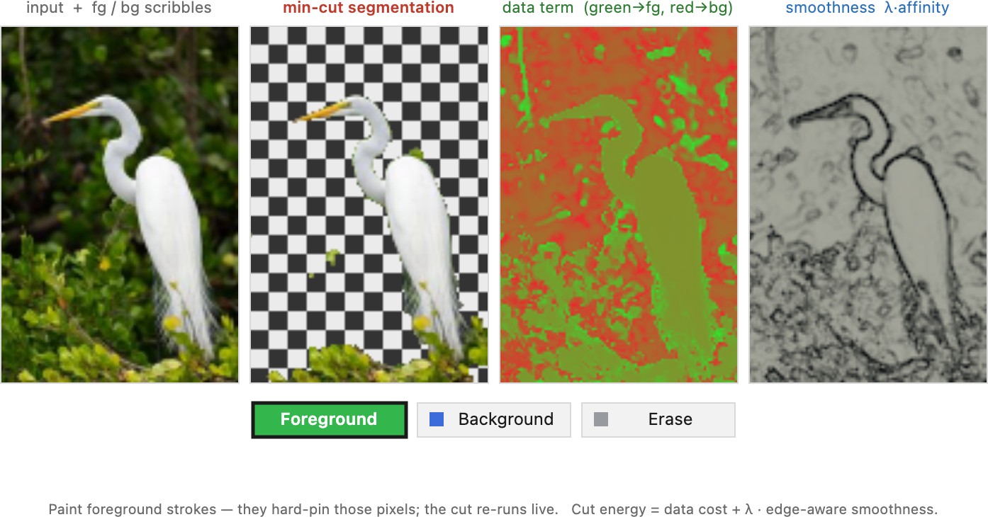
The cleanest framing is Boykov and Jolly's (2001) interactive graph cut. Treat the image as a grid graph whose nodes are pixels, and let the user paint a few foreground and background strokes. From those strokes build a color model (the color distribution of foreground pixels versus background pixels) which gives a per-pixel data term $D_p(L_p)$: the cost of labeling pixel $p$ foreground or background, low when $p$'s color matches that label's model. Add the edge-aware smoothness term
a penalty for giving neighboring pixels $p,q$ different labels: large (expensive to cut) when their colors are similar, small (cheap to cut) when their colors already differ. The total energy is
For binary labels and nonnegative Potts pairwise weights, this energy can be minimized exactly by an s–t cut. The guarantee is conditional on fixed data terms and this submodular pairwise form; arbitrary binary energies need not admit the same construction. Enforce user labels with hard constraints or penalties larger than any possible saving elsewhere.
With fixed costs and nonnegative binary Potts interactions, min-cut finds the global energy minimum. The selected boundary is only as appropriate as the costs and constraints. Color affinity makes some boundaries cheaper; it does not establish object identity.
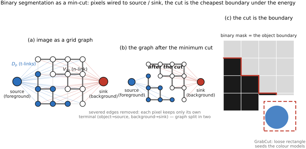
GrabCut alternates Gaussian-mixture color-model fitting and graph-cut labeling, typically initialized from a rectangle (Rother et al. 2004). Outside pixels are background; inside pixels remain candidates for either label. Each fixed-model cut is optimal for its energy, but the joint alternating procedure is not guaranteed to reach a global optimum. User strokes can repair a poor initialization.
Normalized cuts penalize graph cuts relative to the association, or weighted degree, of each group (Shi & Malik 2000). A generalized eigenvector solves a continuous relaxation; thresholding it does not guarantee the exact discrete optimum. Intelligent scissors finds a low-cost path between user anchors, usually with Dijkstra's algorithm on nonnegative edge costs (Mortensen & Barrett 1995). It traces a boundary rather than fitting a region-color model.
Graph-cut segmentation and colorization both use image-dependent relationships between pixels, but their variables, costs and solvers differ. Set the two energies side by side. Binary segmentation minimizes
which charges $w_{pq}$ each time neighbors take different labels. Colorization (Chapter 10.3, Edge-preserving optimization — colorization) minimizes
over a continuous chroma $U$, with the scribbled pixels held fixed. In both, a high affinity $w_{pq}$ between similar neighbors makes it expensive for them to disagree, so the answer changes mostly across edges. The first is a discrete problem solved exactly by min-cut when the pairwise term is submodular; the second is quadratic and reduces to a sparse linear system. The weights in the two are defined and normalized differently, so they are not interchangeable. Closed-form matting introduces another specific local color model; replacing a binary label with a continuous variable does not derive it automatically (Chapter 10.5, Matting Laplacian).
For a practical selection, use a suitable interactive or learned segmenter, inspect missed objects and holes, then construct an uncertainty band for matting where needed. Promptable models such as SAM can provide candidate masks (Kirillov et al. 2023); their boundary confidence is not fractional optical coverage. Preserve editable masks and inspect a replacement background at final output size.
To build the binary cut graph, add source and sink terminals and assign foreground to the source side. Connect the source to pixel $p$ with capacity $D_p(\mathrm{background})$, and $p$ to the sink with capacity $D_p(\mathrm{foreground})$. Whichever side contains $p$, the cut pays the data cost for that label. A neighbor edge of capacity $\lambda V_{pq}$ is cut only when the two pixels receive different labels. Thus the cut cost is exactly the stated energy. The construction explains both the speed of using an existing max-flow solver and the restriction on the energy it solves.
These methods also differ in what the user supplies. Intelligent scissors uses boundary anchors; seeded graph cuts use examples of region membership; GrabCut can begin with a rectangle. Reducing interaction means asking the model to infer more. It does not eliminate ambiguity when foreground and background look alike.
Recap: big lessons of this chapter
With fixed costs and nonnegative binary Potts interactions, min-cut finds the global energy minimum. The selected boundary is only as appropriate as the costs and constraints. Color affinity makes some boundaries cheaper; it does not establish object identity.