6.4 Sampling, downsampling, and aliasing⧉
A camera integrates light over each pixel’s spatial footprint and exposure interval, then records those measurements on a grid. We can model this as filtering followed by point sampling. The filtering reduces fine detail, but generally does not remove every frequency the grid cannot resolve. Resizing introduces another sampling step and another opportunity for aliasing. Chapter 6.5, Resampling and upsampling treats reconstruction between samples; here we examine the information lost or confused by the sampling grid.
6.4.1 Aliasing: a high frequency in disguise⧉
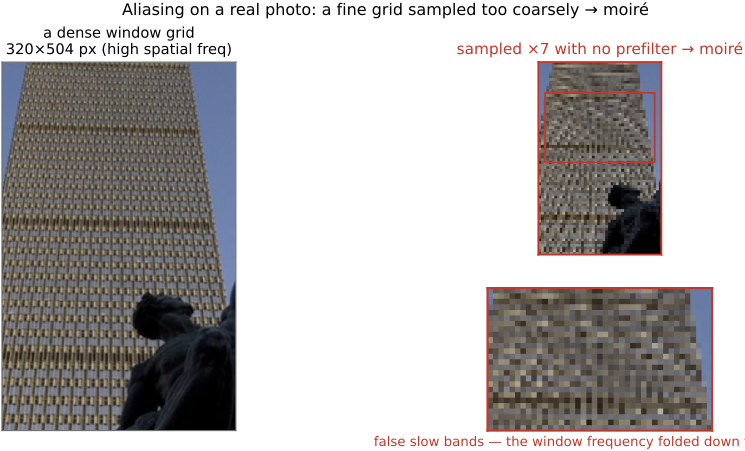
Picture photographing a building's facade (rows of fine windows, or a striped shirt) and shrinking the result. Where the stripes are finer than the output pixels, they do not melt into a uniform gray; they reorganize into bold, wrong, low-frequency bands and swirls that are not in the scene at all: moiré. Intuitively, when a pixel must summarize detail it cannot represent, it ought to return the local average, a neutral gray. Instead, the leftover high frequency gets misread as a low one.
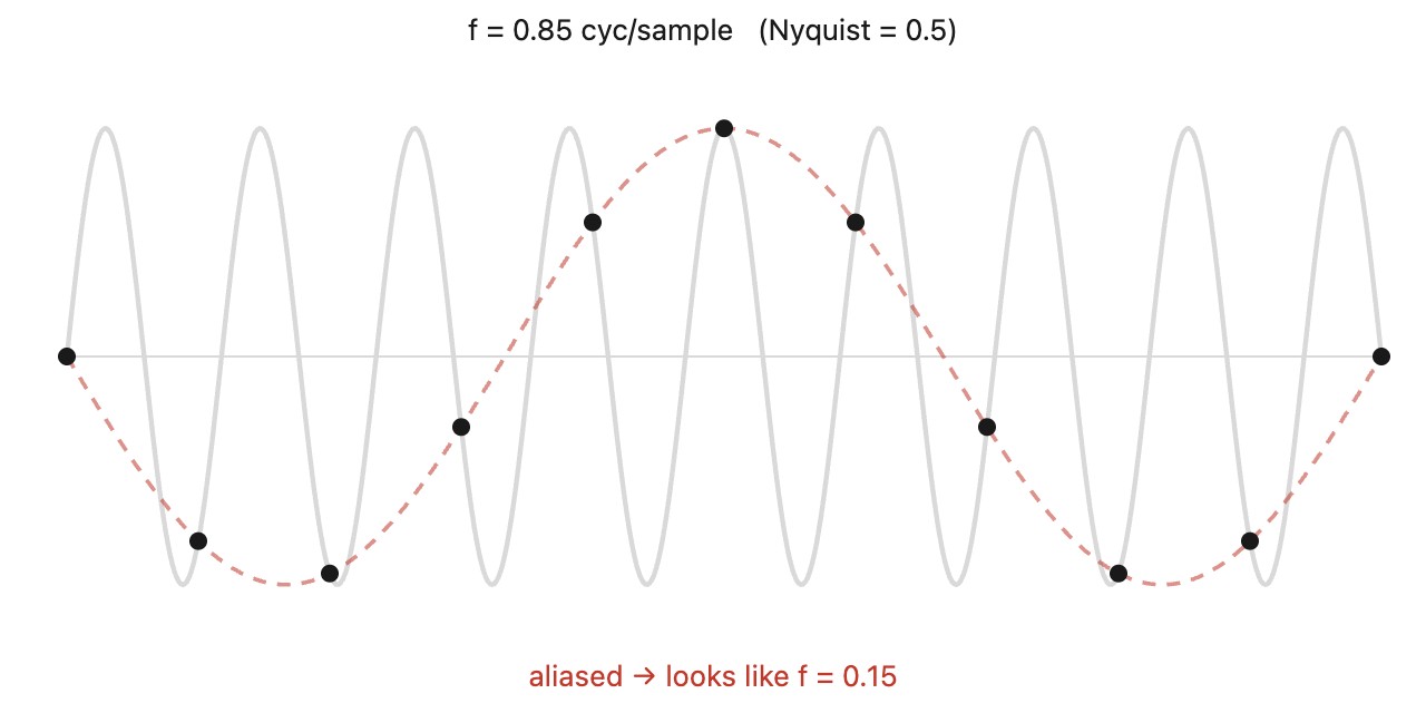
The clean case is a single sine wave (Figure 6.4.1). Sample a high-frequency sine too coarsely (fewer than two samples per cycle) and the samples you collect fall into a pattern indistinguishable from a lower-frequency sine. The original travels in disguise as a different frequency; that impostor frequency is its alias. The damage is not blur (lost detail you could shrug off); it is corruption: energy that lands at the wrong frequency and masquerades as real structure. The same masquerade plays out in 2-D on a real photograph (Figure 6.4.2): a facade's regular window grid is a high spatial frequency, and sampling it too coarsely without a pre-filter folds that grid down into bold, slow moiré bands that are not in the building.
6.4.2 Nyquist and the sampling theorem⧉
For an ideal band-limited signal with highest frequency $f_{\max}$, uniform samples at rate $f_s>2f_{\max}$ determine the signal exactly. The Nyquist frequency is $f_s/2$. The strict inequality avoids the boundary case: a sine exactly at Nyquist can vanish at every sample for one phase. The theorem assumes an unlimited sequence of exact samples; finite, noisy measurements require further choices.
Frequencies separated by an integer multiple of the sampling rate produce identical complex samples:
For example, at 100 samples per unit length, cosines at 70 and 30 cycles per unit length give the same samples. A lone sampled image cannot distinguish them without assumptions. Additional shifted measurements or a restrictive scene model can resolve some ambiguities; applying a blur afterward cannot generally separate components already mixed by aliasing.
Sample above twice the highest retained frequency. If the signal is too detailed for the grid, low-pass it before sampling. This applies to space and time. Real prefilters have finite transition bands, so allow a margin below Nyquist and check residual aliasing.
The theorem cuts both ways, which is why it is so central. It tells you when sampling is safe (the signal is already band-limited below Nyquist, so nothing folds) and exactly what to do when it is not: kill the offending frequencies before they fold. And because it is a statement about any sampled signal, it reappears far beyond image shrinking: in audio (the 44.1 kHz CD rate is a little over twice the ~20 kHz of human hearing), in video frame rates, and (on the time rather than the space axis) as the temporal aliasing we just named.
6.4.3 In two dimensions, aliasing has a direction⧉
On a rectangular 2-D grid, aliasing folds each frequency coordinate by the sampling rate along that axis. A frequency vector can therefore change both length and orientation. A purely vertical grille does not acquire an arbitrary diagonal orientation on an aligned rectangular grid; both frequency coordinates and the grid geometry determine the alias.
A sharp slanted edge contains arbitrarily high frequencies perpendicular to the edge. Point-sampling it produces a staircase whose pattern depends on its position relative to the grid. Pixel-area integration softens the staircase, though a box footprint is not an ideal band limit. Rendering and image reduction use the same prefiltering principle.
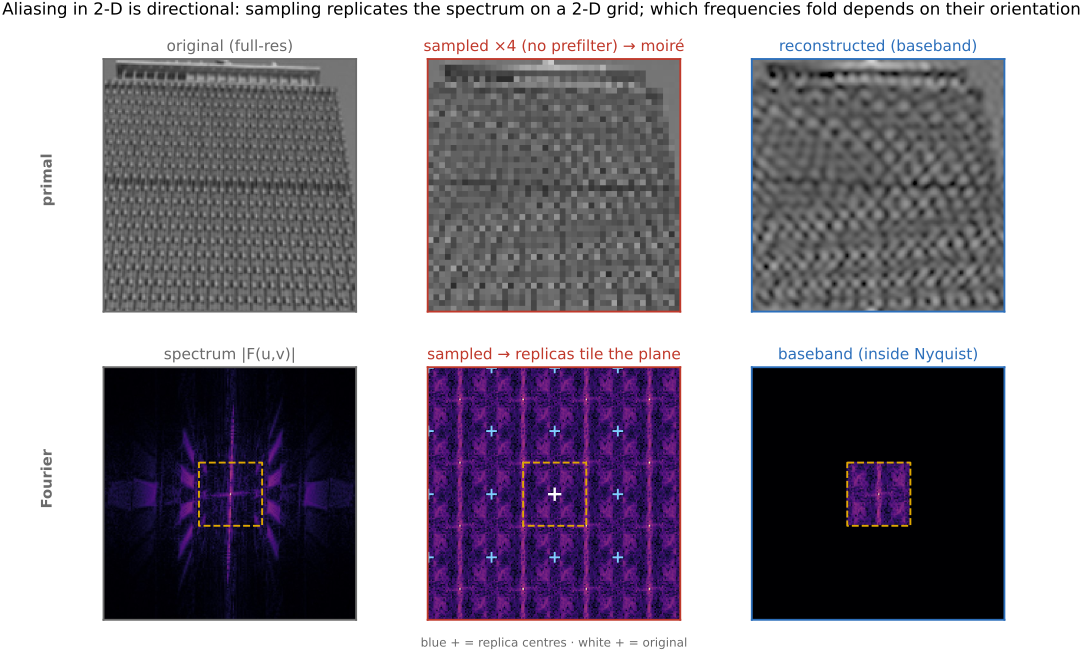
For example, sample a sinusoid with frequency components 0.6 cycles per pixel horizontally and 0.2 vertically on an integer pixel grid. Subtracting one horizontal cycle per pixel changes its frequency vector to (−0.4, 0.2) without changing the samples: the phase difference at every integer horizontal coordinate is a whole number of cycles. The apparent orientation changes because the horizontal component has folded while the vertical component has not. A regular texture containing several frequency components can therefore produce moiré at orientations absent from the visible coarse structure of the original texture.
6.4.4 Sampling in the frequency domain: spectral replicas⧉
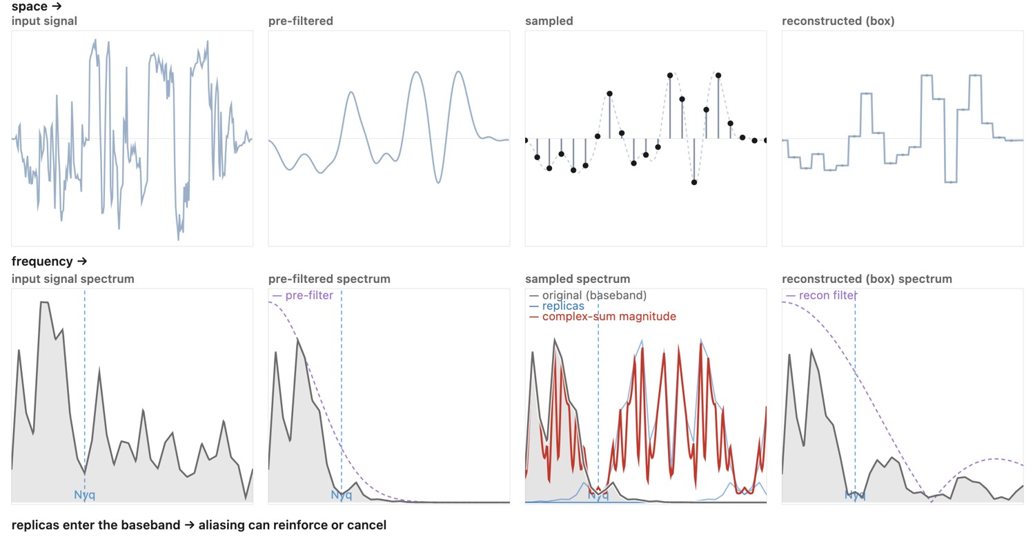
In the frequency domain the mechanism is vivid. Sampling on a grid is multiplying the signal by a comb of spikes, and multiplying by a comb in space replicates the spectrum: it pastes shifted copies of the signal's spectrum at every multiple of the sampling rate. If the original spectrum is narrow enough (band-limited below Nyquist), the copies sit side by side without touching and the original can be isolated. If it is too wide, the copies overlap, the tails fold back over the genuine low frequencies, and that overlap is aliasing. Seen this way the fix is obvious: band-limit the signal before you sample it. Run a low-pass filter (a blur) first, to delete the frequencies above Nyquist that would otherwise fold, then sample. This pre-filter (anti-aliasing) trades a little sharpness for the removal of false structure, and it is why a well-written image-shrinking routine blurs before it downsamples. The space-versus-frequency tradeoff returns: a perfectly sharp cutoff in frequency is a sinc spread out forever in space, so practical pre-filters compromise.
Figure 6.4.4 draws the multiplication in space first, then the replicated spectrum it produces.
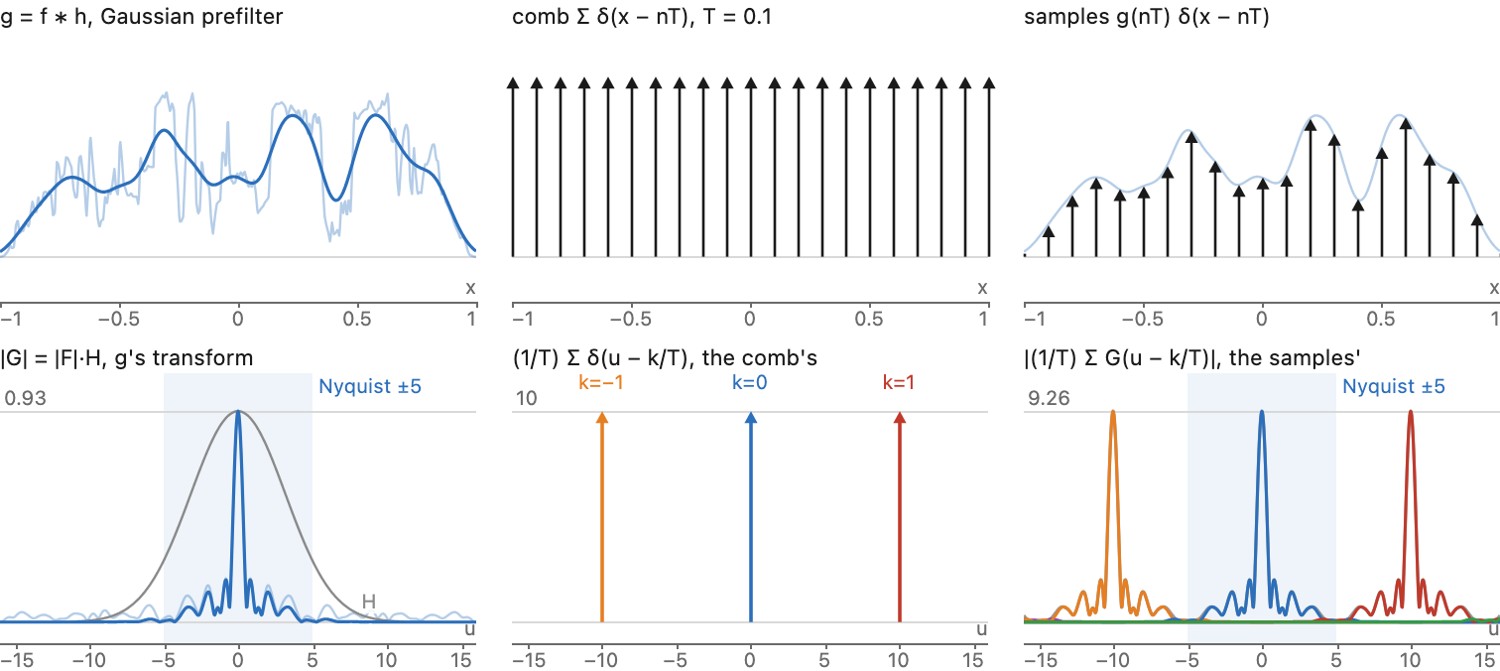
Sampling on a grid is multiplication by a comb (a train of deltas), and a comb's Fourier transform is another comb, so sampling replicates the signal's spectrum at every multiple of the sampling rate. If the spectrum is band-limited below Nyquist the copies sit side by side and the original is recoverable; if it is not, the copies overlap, and the folded-over tails land on top of the genuine low frequencies as aliasing: energy appearing at completely wrong frequencies (moiré, the backward wagon-wheel). The cure is to band-limit before sampling: low-pass away everything above Nyquist first, then sample.
6.4.5 Seeing it: sampling and pre-filtering, hands on⧉
The demos below show this directly. The first demo is the one-dimensional story (a single signal, your hand on the sampling rate), and the second is the two-dimensional one, the same physics on a real photograph where aliasing shows up as moiré.
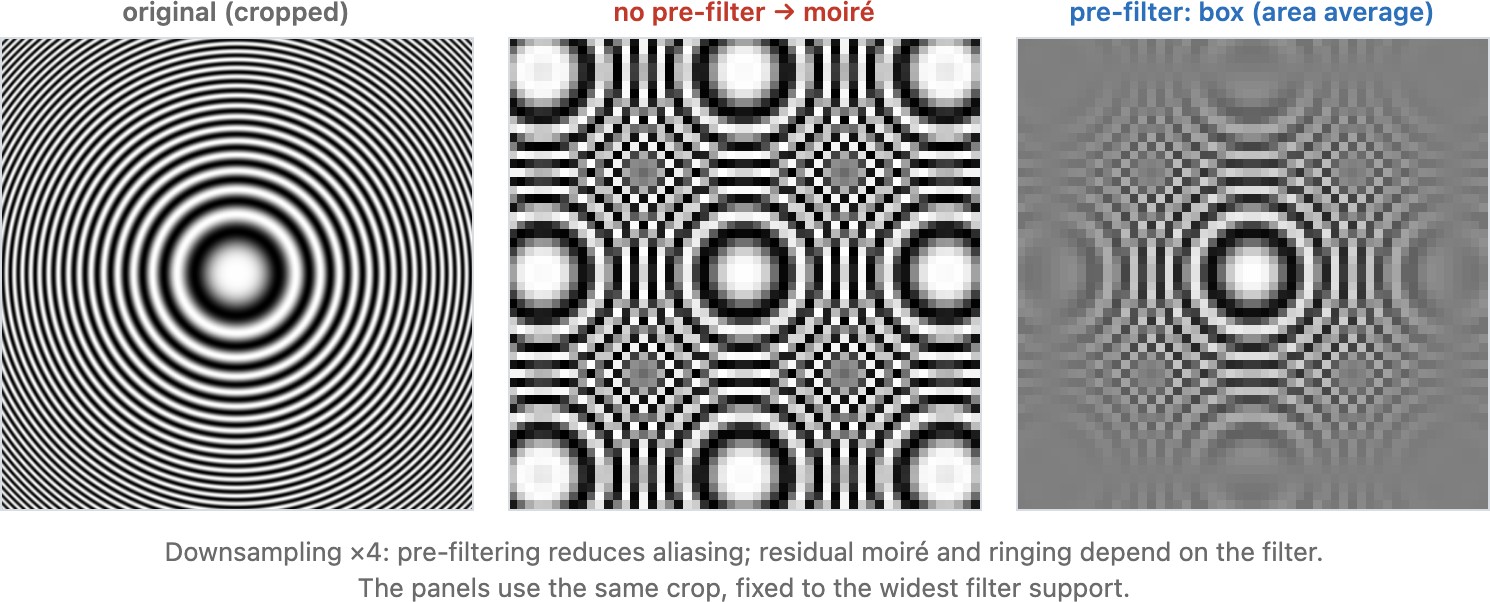
The full sampling pipeline generalizes to two dimensions just as cleanly, and the spectral picture is the most revealing part: in 2-D, sampling replicates the spectrum on a whole lattice of copies, and aliasing is a copy drifting in to overlap the baseband.
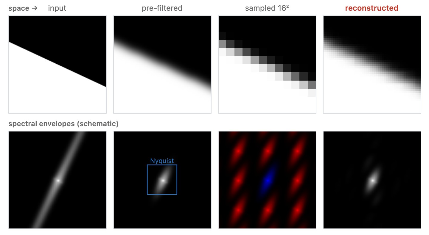
Two continuous signals that agree at every point sample are indistinguishable on that grid. A sensor pixel averages a spatial footprint instead, which attenuates some fine variation before the grid samples it. That helps, but a box average has spectral side lobes and does not eliminate all aliases. The footprint and the sample spacing are separate parts of the model.
Moiré can also measure the relative displacement of two known fine patterns: a small change in alignment moves their broad beat pattern. The known pattern supplies information absent from arbitrary-image reconstruction. A related printed-animation example is KineCAM, which interleaves captured frames into a kinegram viewed through a striped overlay. It does not recover camera pose from sensor-grid moiré.
6.4.6 The ideal reconstruction filter: sinc, and why it is unreachable⧉
For uniform spacing $T=1/f_s$, ideal reconstruction of a signal band-limited below Nyquist is
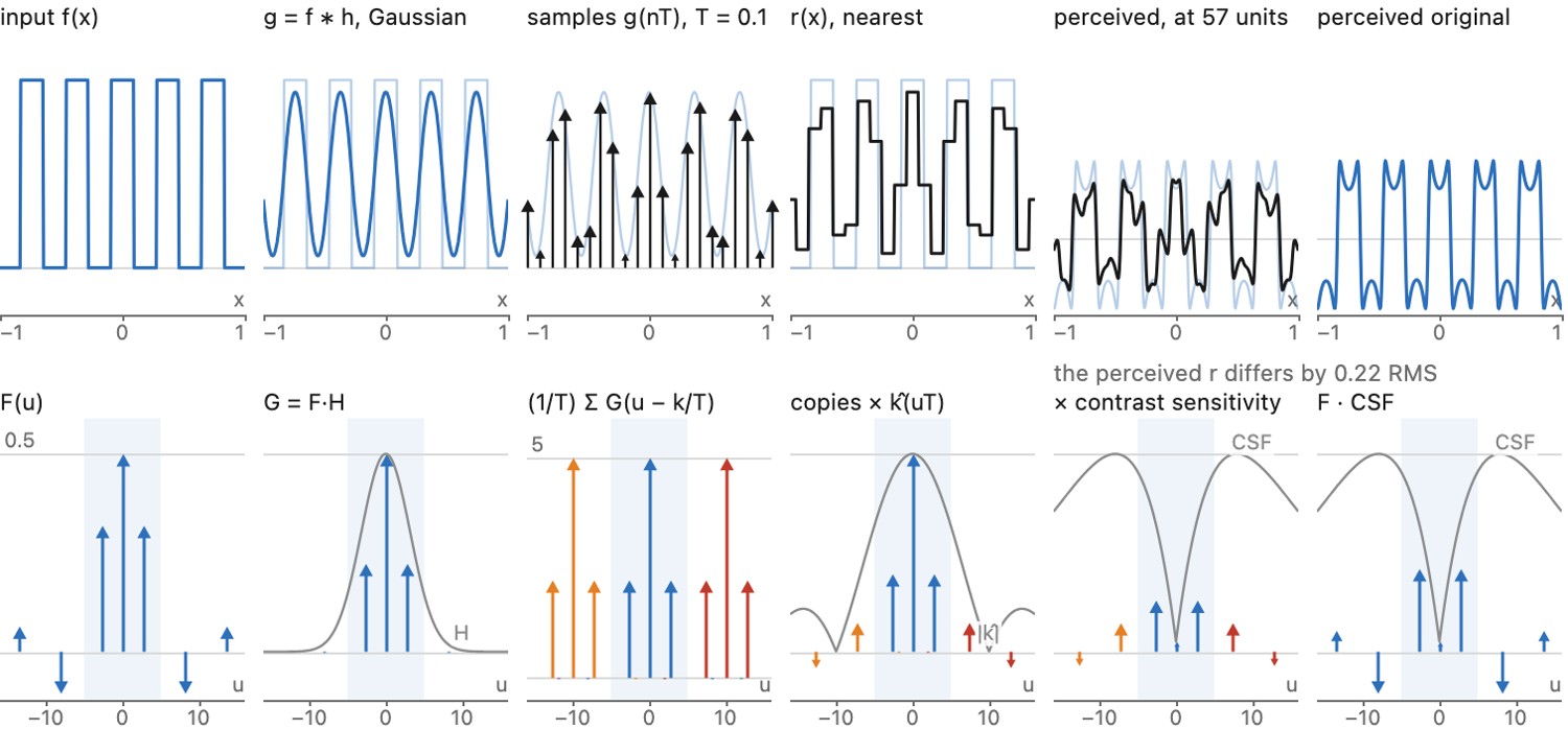
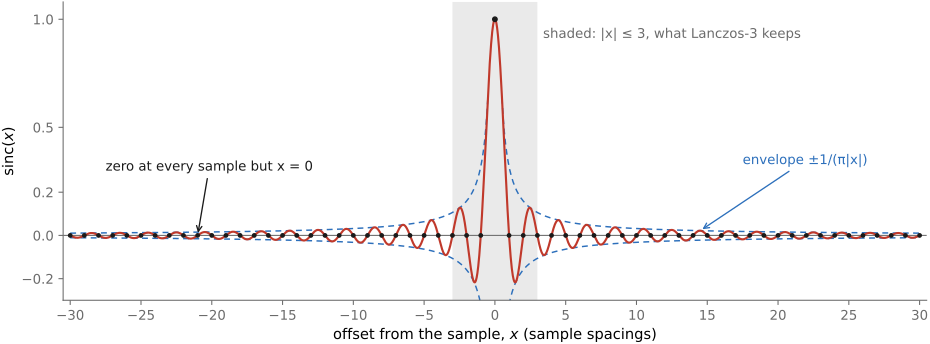
Each sample contributes a shifted sinc. At the sample locations, every other sinc is zero. The infinite sum makes exact reconstruction impractical for a finite image. Practical kernels limit support and trade passband attenuation, stopband leakage, and ringing. Sharp low-pass filtering can overshoot an edge even before truncation; truncation is not the sole cause. Chapter 6.5, Resampling and upsampling develops the usable kernels.
Ideal band limiting and ideal interpolation use sinc kernels, scaled for their respective grids. Their infinite support requires approximation in finite computations. A finite filter trades computation and frequency selectivity; inspect both aliasing and edge overshoot.
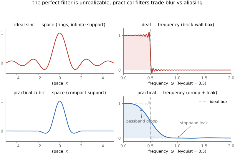
Figure 6.4.9 puts the whole chain in one place, one column per step: the input, the prefilter, the samples, the reconstruction, and the reconstruction as a viewer perceives it.
6.4.7 Practical filters: from the box to bicubic and Lanczos⧉
Downsampling needs a prefilter, and the previous section named the ideal one: a sinc scaled to the output spacing, whose transform is a box that keeps every frequency the coarser grid can hold and removes all the others. The sinc cannot be used as it is. It is infinitely wide, so every output pixel would read the whole image, and its lobes decay so slowly that truncating it changes its response, while its negative lobes overshoot at edges (Figure 6.4.10). Every practical prefilter is therefore a finite kernel that approximates it. The crudest is the box: averaging each $q\times q$ block of pixels into one output pixel, the usual way to halve an image. Its transform is itself a sinc, which keeps only 0.64 of the signal at the new Nyquist frequency and lets through as much as a fifth beyond it. The tent and the Gaussian are smoother, and the cubics and the Lanczos windowed sinc come closest to the ideal. The same kernels, used at the input's spacing rather than the output's, reconstruct a continuous image from its samples, which is how upsampling uses them (Chapter 6.5, Resampling and upsampling), and the trade-offs below hold for both uses.
So every practical prefilter or reconstruction kernel is an approximation of sinc with finite support, balancing two competing evils that are clearest in the frequency domain (Figure 6.4.8). A kernel that is too gentle loses medium frequencies (its response rolls off early and the image goes soft), while one too aggressive lets high frequencies alias: it leaks past the grid's limit and admits jaggies and moiré. Every kernel is a point on this blur-versus-alias tradeoff. The two famous families both live on it.
Fourier analysis says the perfect reconstruction and anti-aliasing filter is the sinc, a perfect box in frequency. But the sinc is infinitely wide and rings when truncated, so no real filter can be it. Every practical kernel (bilinear, bicubic, Lanczos) is a deliberate compromise between approximating that idealized sinc (what Fourier wants) and staying compactly supported (what computation, and ringing, demand): reach wider and you approach sinc; truncate harder and it gets cheaper and less ringy but further from ideal.
Read off the frequency response, the same compromise is a tug-of-war between two errors. Passband droop: a too-gentle filter attenuates frequencies below Nyquist that the grid could have represented, so the image goes soft. Stopband leak: a too-aggressive filter lets frequencies above Nyquist through, which alias into jaggies and moiré. A good kernel sits at the sweet spot (flat passband up to Nyquist, sharp rejection beyond) and box, tent, bicubic and Lanczos are just different points on this droop-versus-leak curve.
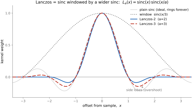
Lanczos is sinc literally windowed by a wider sinc:
over a support of $a$ samples on each side (and zero beyond, with $k(0)=1$). It hugs the ideal closely and looks crisp, at the cost of some ringing near strong edges, the surviving side-lobes of the truncated sinc (Figure 6.4.11).
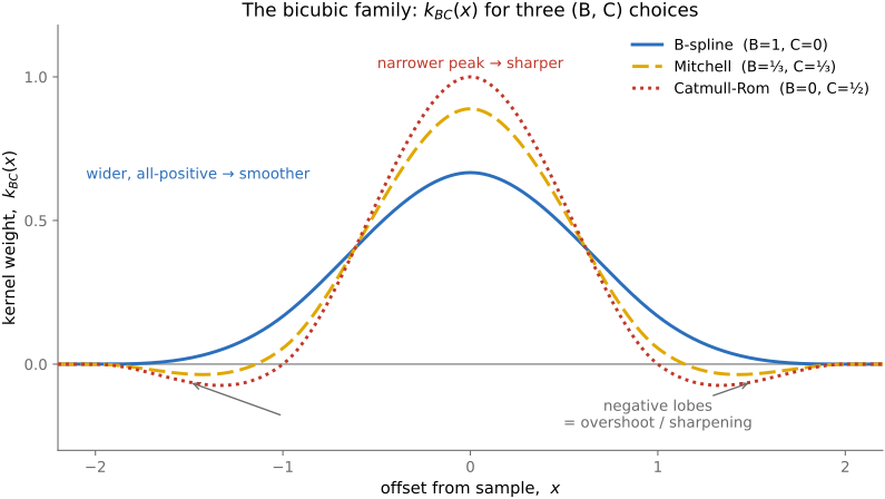
Bicubic uses a piecewise cubic polynomial: smooth, compact (four samples wide in 1-D), the standard default in image editors. It typically carries small negative lobes to the sides, and those are not a bug: they give the reconstruction a built-in mild sharpening (much like the unsharp mask) that makes upscaled images crisper. The cubic kernel is not unique: there is a family. Once you impose the natural requirements (the kernel should be symmetric, should be smooth where the cubic pieces meet, and should sum to one so it preserves brightness), a cubic still has two free parameters left. Mitchell and Netravali (1988) named them $B$ and $C$ (an open-access summary with the kernel formula is the Wikipedia article on Mitchell–Netravali filters); the result is a single piecewise cubic, supported over four samples (two on each side):
one cubic whose two knobs slide it between sharper and smoother. Three points of the $(B,C)$ plane are the canonical members worth knowing by name:
- $(B,C)=(1,0)$, the cubic B-spline: the smoothest member, all-positive (no negative lobes), and approximating rather than interpolating, so it visibly blurs;
- $(B,C)=(0,\tfrac12)$, Catmull–Rom: interpolating (it passes exactly through the samples) with pronounced negative lobes, so it looks sharp;
- $(B,C)=(\tfrac13,\tfrac13)$, Mitchell–Netravali: the balanced default, sitting between the two and chosen as a useful compromise among visible artifacts.
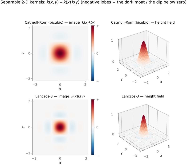
A separable 2-D kernel $k(x)k(y)$ generally treats axes and diagonals differently. The continuous Gaussian is both separable and radially symmetric; truncation on a square only approximates that symmetry. For a rectangular sampling lattice, ideal rectangular-band reconstruction uses a separable product of sincs. It is not radially symmetric. A circular passband has a radial jinc kernel and discards some frequencies allowed near the corners of the rectangular Nyquist region.
The cubic-convolution filters used here evaluate a fixed piecewise-cubic kernel at fractional offsets and sum weighted samples. They do not solve a regression for every output pixel. Other methods also called bicubic interpolation use polynomial or spline constructions; the name alone does not identify the algorithm or its downsampling behavior.
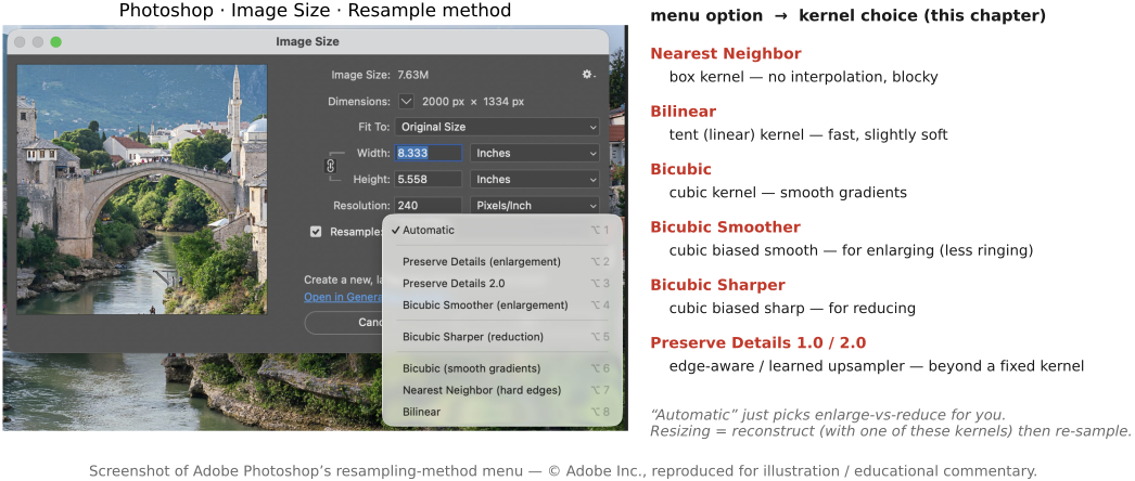
Mitchell and Netravali (1988) found their balance by running a perceptual study mapping which $(B,C)$ choices look best, charting where each lands among three failure modes: residual blur (too little negative lobe), ringing (ghost edges from too-strong negative lobes), and anisotropy (a visible preference for the horizontal / vertical / diagonal directions). A broad region of the $(B,C)$ map looks satisfactory, but different points suit different images, which is exactly why Photoshop and friends offer you a choice of bicubic ("bicubic smoother" for enlargements, "bicubic sharper" for reductions) rather than one fixed filter. There is no universally best answer, only a tradeoff you tune to the image: a slightly blurry original can afford a sharper kernel, a crisp one cannot.
Real software exposes exactly these kernel choices. Photoshop's Image Size resample menu lets you pick Nearest Neighbor, Bilinear, Bicubic, Bicubic Smoother (for enlargements), Bicubic Sharper (for reductions), and Preserve Details: the very box / tent / cubic family, and the smooth-versus-sharp bicubic tradeoff, turned into a dropdown (Figure 6.4.14).
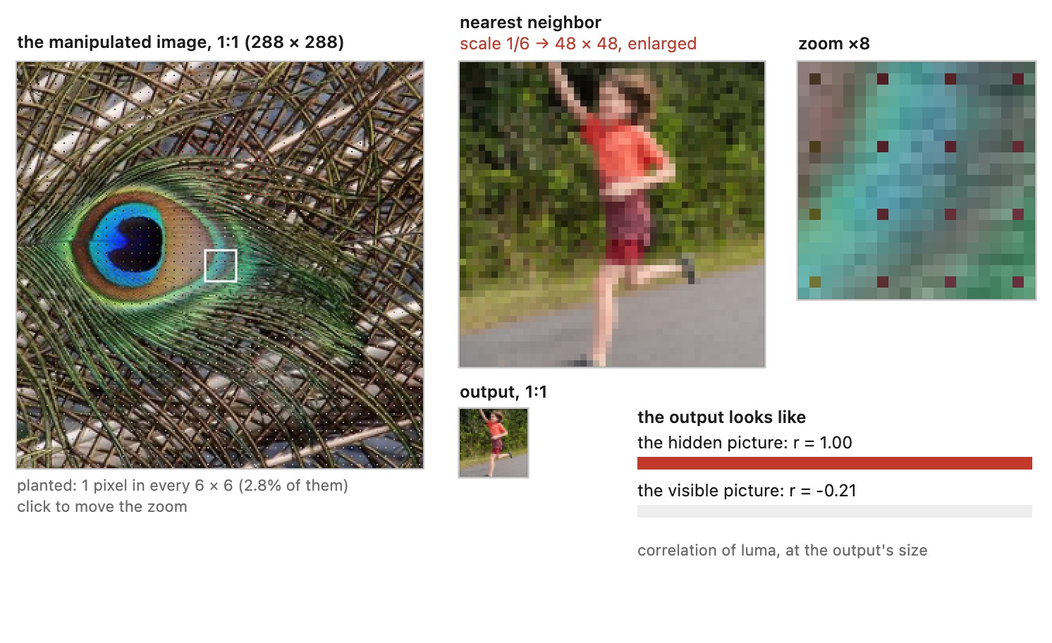
Specify the cubic kernel, coordinate convention, boundary rule, and whether its support widens during reduction. Two libraries can both say “bicubic” and produce different results. Resizing differences can substantially alter generative-model evaluation (Parmar et al.). Scaling is also part of an adversarial attack surface (Gao et al.); the simple nearest-neighbor example below illustrates one mechanism, not the full class of attacks.
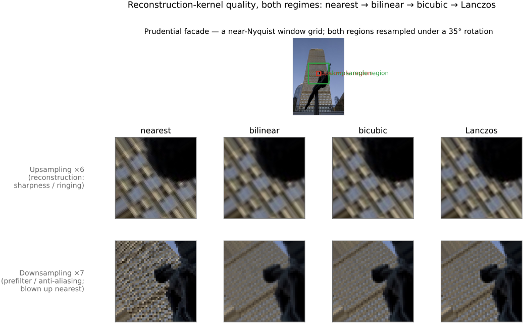
A separable kernel is cheap because a horizontal one-dimensional operation followed by a vertical one replaces a full two-dimensional neighborhood sum. The price can be directional behavior. Rotate a slanted edge while keeping the sampling grid fixed and compare the result: a square product footprint can treat the axis-aligned and diagonal cases differently. The continuous Gaussian shows that separability and radial symmetry can coexist, because the product of its two one-dimensional exponentials depends only on squared radius. A product of sinc kernels instead corresponds to the rectangular frequency region of the sampling grid. Choosing a circular footprint changes that region; it is not merely a more accurate implementation of the same filter.
Recap: big lessons of this chapter
Sample above twice the highest retained frequency. If the signal is too detailed for the grid, low-pass it before sampling. This applies to space and time. Real prefilters have finite transition bands, so allow a margin below Nyquist and check residual aliasing.
Sampling on a grid is multiplication by a comb (a train of deltas), and a comb's Fourier transform is another comb, so sampling replicates the signal's spectrum at every multiple of the sampling rate. If the spectrum is band-limited below Nyquist the copies sit side by side and the original is recoverable; if it is not, the copies overlap, and the folded-over tails land on top of the genuine low frequencies as aliasing: energy appearing at completely wrong frequencies (moiré, the backward wagon-wheel). The cure is to band-limit before sampling: low-pass away everything above Nyquist first, then sample.
Ideal band limiting and ideal interpolation use sinc kernels, scaled for their respective grids. Their infinite support requires approximation in finite computations. A finite filter trades computation and frequency selectivity; inspect both aliasing and edge overshoot.
Fourier analysis says the perfect reconstruction and anti-aliasing filter is the sinc, a perfect box in frequency. But the sinc is infinitely wide and rings when truncated, so no real filter can be it. Every practical kernel (bilinear, bicubic, Lanczos) is a deliberate compromise between approximating that idealized sinc (what Fourier wants) and staying compactly supported (what computation, and ringing, demand): reach wider and you approach sinc; truncate harder and it gets cheaper and less ringy but further from ideal.
Read off the frequency response, the same compromise is a tug-of-war between two errors. Passband droop: a too-gentle filter attenuates frequencies below Nyquist that the grid could have represented, so the image goes soft. Stopband leak: a too-aggressive filter lets frequencies above Nyquist through, which alias into jaggies and moiré. A good kernel sits at the sweet spot (flat passband up to Nyquist, sharp rejection beyond) and box, tent, bicubic and Lanczos are just different points on this droop-versus-leak curve.
The cubic-convolution filters used here evaluate a fixed piecewise-cubic kernel at fractional offsets and sum weighted samples. They do not solve a regression for every output pixel. Other methods also called bicubic interpolation use polynomial or spline constructions; the name alone does not identify the algorithm or its downsampling behavior.