45.2 Refreshers🔗⧉

The whole book runs on a handful of mathematical ideas, reused relentlessly. Images are vectors; many useful operations are linear maps, which lets us borrow all of linear algebra and the Fourier transform; recovering an image from imperfect measurements is an optimization problem: fit the data and impose a prior; probability models the noise; learned methods now handle many tasks. This appendix is that kit. Each section sketches one tool just far enough to read the chapters that use it, always with an eye on the imaging use, and points you to where to go deeper. It is deliberately tight: lean on the figures, and defer the proofs to the texts named in each section.

45.2.1 Linear algebra🔗⧉

Vectors and matrices are the native language of imaging. A pixel grid is a vector; a blur, a color transform, a resampling is a matrix; and many imaging problems involve solving a linear system, either directly or inside a nonlinear solver. The main idea in this section is the orthogonal basis: a coordinate system in which a hard operator becomes easy.

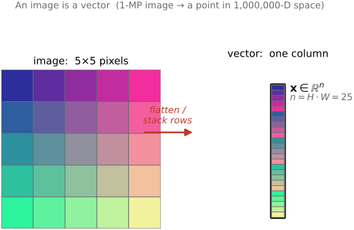
An image is a vector. A vector is just a length-$n$ list of numbers, which you can also picture as a point, or an arrow from the origin, in $n$-dimensional space. The book's basic move is to treat an image as one of these: stack its pixels into a single tall column (Figure 45.2.1⛶ fullscreen). A one-megapixel grayscale photo is then a single point in a million-dimensional space, and everything we do to it (brighten, blur, sharpen, denoise) is geometry in that space. (Stacking is sometimes literal, in the code, and sometimes just a way to think; either way the algebra is the same.)

Inner product, norm, angle. The inner product $\langle u,v\rangle = u^\top v$ measures how much two vectors align; the norm $\|v\| = \sqrt{\langle v,v\rangle}$ is length; and $\langle u,v\rangle = 0$ means orthogonal (perpendicular). This one operation does an enormous amount of imaging work: it is how a cone "reads" a spectrum (project the spectrum onto the cone's sensitivity), how a filter responds to a patch, and how we measure the similarity between two images. Keep "inner product = how much of this is in that" as the intuition.

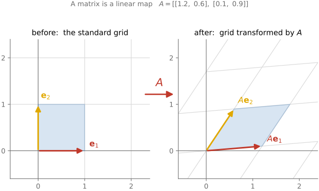
Matrices are linear maps. Write $y = Ax$: a matrix sends a vector to a vector, linearly: it respects sums and scaling, $A(\alpha x_1 + \beta x_2) = \alpha A x_1 + \beta A x_2$. For a $2\times 2$ $A$ you can see exactly what it does by watching it deform the unit square (and the grid around it) into a parallelogram (Figure 45.2.2⛶ fullscreen): rotation, scaling, shear. A fixed blur, fixed-kernel resampling, or known geometric warp can be linear in pixel values. Color conversions may include offsets, making them affine, while estimating the warp itself is generally nonlinear. (One caution from the linear-image-processing chapter: matrix multiplication does not commute, $AB \ne BA$ in general, so the order of operations matters.)

Linear systems and inverse problems. Imaging forward models are read in the $y = Ax$ direction: a clean scene $x$ goes through some physical process $A$ (optical blur, mosaic sampling, projection) to produce a measurement $y$. Recovering $x$ from $y$ is then solving the system, inverting $A$. The catch, which sets up the rest of this appendix, is that $A$ is usually enormous, often rank-deficient (it throws information away: its null space is exactly what the measurement cannot see), and the data is noisy. So we almost never literally invert; we optimize (the next two sections). The vocabulary to keep: square vs over-/under-determined systems, rank, and null space.

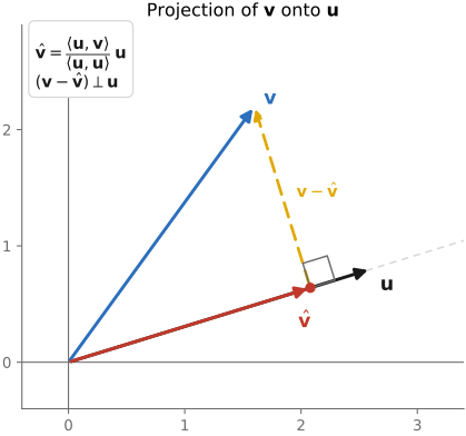
Bases, projection, orthogonality. A basis is a choice of coordinate system; changing basis re-expresses the same vector in new coordinates. Projecting a vector $v$ onto a direction $u$ (its shadow on $u$) is $\hat v = \frac{\langle u,v\rangle}{\langle u,u\rangle}\,u$ (Figure 45.2.3⛶ fullscreen). Bases get dramatically nicer when they are orthonormal (mutually perpendicular unit vectors $\{e_i\}$): then the coordinates are just inner products, $x = \sum_i \langle e_i, x\rangle\, e_i$: no system to solve, and energy is preserved (Parseval: the norm is the same in either basis). This is why orthogonal bases recur throughout the book (Fourier, orthonormal wavelets): they re-coordinatize an image for free. The flip side is a recurring complication in Chapter 4.1, Color space 101: cone sensitivities and display primaries play different roles. Cones measure inner products of spectra with sensitivity functions; display primaries synthesize spectra from coefficients. Neither spans all spectra, and their relationship requires a calibrated color transform. Non-orthogonal bases need dual vectors for coordinate extraction; the distinction between measurement and synthesis matters throughout colorimetry.

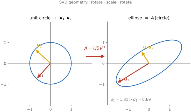
Eigenvectors and the SVD. Some directions a matrix only scales, never rotates: its eigenvectors, with eigenvalues the scale factors. For a real symmetric matrix an orthonormal eigenbasis can be chosen (the spectral theorem), so diagonalizing it means finding the basis where the operator is nothing but per-axis scaling. The singular value decomposition $A = U\Sigma V^\top$ generalizes this to any matrix, even non-square: read it right to left as apply an orthogonal transformation ($V^\top$), scale by the singular values in $\Sigma$, then apply another orthogonal transformation ($U$); these transformations can include reflections. Geometrically, $A$ takes the unit circle to an ellipse whose axes are the singular values (Figure 45.2.4⛶ fullscreen). The SVD underlies low-rank approximation, PCA, the pseudo-inverse (how you "solve" a system that has no exact solution), and the conditioning of deblurring: tiny singular values mean that inverting $A$ divides by something near zero, which is why deconvolution blows up noise (Chapter 6.3, Linearity, Fourier, Aliasing and deblurring).

💡 Big lesson. Whenever possible, express a linear operation in a basis where it is diagonal. The "diagonalize / go to Fourier" maxim that runs through the book (Big Lessons) is, at bottom, this linear-algebra fact, and this section is where it is planted. For the deeper treatment, Strang's Linear Algebra and Learning from Data and chapters 2–4 of Deisenroth, Faisal & Ong are the companions; and for building the geometric intuition behind everything above (vectors, matrices as transforms, projection, the SVD), Immersive Linear Algebra is a free online companion whose 3-D figures you rotate and drag right in the browser.

45.2.2 Calculus: derivatives, gradients, integrals🔗⧉

Three calculus ideas earn their keep in imaging. Derivatives measure change, so intensity changes mark edges. Gradients point uphill, so a suitably sized step along the negative gradient can reduce a loss. Integrals accumulate light, which is what a pixel records. That is most of what we need; the rest is the chain rule, stated once so the machine-learning section can lean on it.

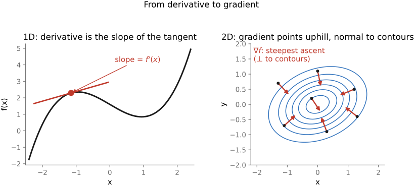
Derivative = slope = rate of change. $f'(x) = \lim_{h\to0}\frac{f(x+h)-f(x)}{h}$ is the slope of the tangent (Figure 6.2.17⛶ fullscreen, left). In a discrete image we approximate it with a finite difference (one pixel minus its neighbor), and that difference is large exactly where intensity changes fast, i.e. at edges. This is the whole basis of Sobel gradients, edge detection, and unsharp sharpening (Chapter 6.2, Convolution).

Partial derivatives and the gradient. For a function of several variables $f(x_1,\dots,x_n)$, the gradient $\nabla f = (\partial f/\partial x_1, \dots, \partial f/\partial x_n)$ stacks the partials into a vector. It points in the direction of steepest ascent, and its length tells you how steep (Figure 6.2.17⛶ fullscreen, right: arrows climbing a contour map). For an image, the gradient at a pixel points across the edge: its direction is normal to the edge and its magnitude is the edge strength.

Jacobian and Hessian: the multivariable second order. Two more objects appear the moment a function takes or returns vectors. A map that sends a vector to a vector, $\mathbf f:\mathbb R^n\to\mathbb R^m$, has a Jacobian $J$, the $m\times n$ matrix of all first partial derivatives, $J_{ij}=\partial f_i/\partial x_j$. It is the best linear approximation of $\mathbf f$ near a point (for a scalar function the Jacobian is the transpose of a column-vector gradient), and composing two maps multiplies their Jacobians: that is the vector form of the chain rule that backpropagation runs on, and the way a geometric warp is linearized locally. When the function is scalar but we care about its curvature, the Hessian $H$ is the $n\times n$ matrix of second partial derivatives, $H_{ij}=\partial^2 f/\partial x_i\partial x_j$. At a point where $\nabla f=\mathbf 0$ the Hessian says which kind of stationary point it is: positive-definite (curving up in every direction) means a genuine minimum, indefinite means a saddle. It is also what second-order optimizers exploit: Newton's method takes the step $-H^{-1}\nabla f$ instead of a fixed $-\eta\,\nabla f$, folding the local curvature into the step. In practice you meet the Jacobian constantly (anywhere a warp or a network is linearized) and the Hessian more rarely, mostly to reason about minima.

Chain rule. The derivative of a composition: $\frac{d}{dx}f(g(x)) = f'(g(x))\,g'(x)$. This unassuming rule is the engine of backpropagation. A deep network is a long composition of functions, and training it means differentiating a loss back through that whole stack: repeated chain rule, applied automatically. We state it here so the ML section can simply invoke it.

Integrals = accumulation. An integral is area under a curve, a continuous sum. In imaging this is not abstract: a pixel value is an integral, the scene's radiance accumulated over the sensor element's area, over the cone of incoming directions, over the exposure time, and over the spectral response of the color filter (Chapter 2.2, Image formation and linear perspective). We constantly slide between the continuous picture (the integral) and the discrete one (a sum over samples): that slide is exactly what sampling and Chapter 6.5, Resampling and upsampling are about.

Convexity, minima, and why gradients matter. At an unconstrained interior local optimum of a differentiable function, $\nabla f=0$; zero gradient can also occur at a saddle or other stationary point. If the function is convex (bowl-shaped, no false bottoms) then $\nabla f = 0$ pins down the global minimum, and gradient methods can converge under suitable step-size and regularity conditions. That is the bridge to the next section: optimization is "follow the negative gradient until the gradient is zero."

💡 Big lesson. Many imaging quantities are multiplicative (illumination $\times$ reflectance, or contrast as a ratio), and taking a $\log$ turns those products into sums and turns derivatives into relative (percentage) change. That is one reason log space keeps reappearing, from exposure stops to tone mapping (Big Lessons). For the calculus itself, chapter 5 of Deisenroth, Faisal & Ong (vector calculus, aimed at exactly this use) is the companion.

45.2.3 Optimization and regression🔗⧉

Most computational-photography problems have the same form: "find the image, or the parameters, that best explain the measurements." Concretely, minimize a loss that is a data-fit term plus a prior. Two tools cover the ground, least squares (when there's a closed form) and gradient descent (when there isn't), and regularization is how we keep ill-posed inverse problems from exploding.

The pattern: loss = data term + prior. Almost every recovery problem has the shape

Denoising, deblurring, demosaicking, HDR merging, white balance: same skeleton every time, only the forward operator $A$ and the prior $R$ change. Recognize this and half the book's algorithms become variations on one theme.

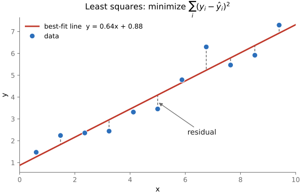
Least squares and the normal equations. Fitting a model (a line, a plane, a response curve) by minimizing the sum of squared residuals (Figure 45.2.5⛶ fullscreen) has a clean closed-form solution, the normal equations $A^\top A\,\hat x = A^\top y$ (and when $A^\top A$ is singular, the SVD-based pseudo-inverse from the last section steps in). Why squared error specifically? Two reasons that recur: it is the maximum-likelihood estimate under Gaussian noise (a tie to the probability section), and squaring keeps the derivative linear, so the math stays tractable. Its weakness (squared error is dominated by a few large residuals, so it is fragile to outliers) is exactly what motivates the robust losses that appear later.

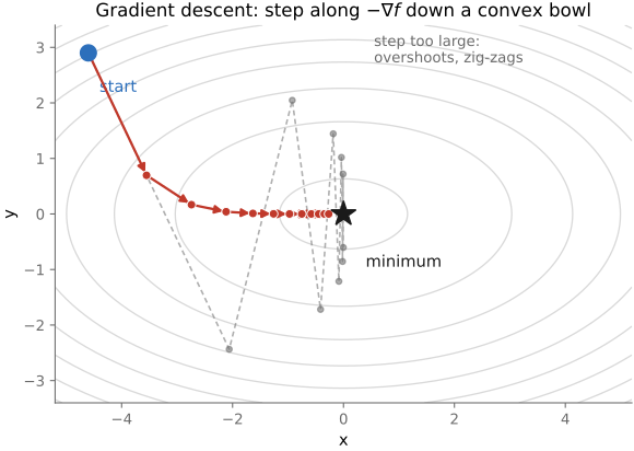
Gradient descent. When the problem is too big for a closed form, or nonlinear, we walk downhill: $x_{t+1} = x_t - \eta\,\nabla f(x_t)$ (Figure 6.9.3⛶ fullscreen). The learning rate $\eta$ is the step size: too large and you overshoot or diverge, too small and you crawl. Three variants in one breath: stochastic gradient descent uses a random minibatch of data per step (how neural nets are actually trained, and why each step is cheap); momentum and Adam smooth and adapt the steps to go faster. For a convex loss every local minimum is global, although it may not be unique and convergence still depends on the algorithm and step size; deep networks are wildly non-convex, full of local minima, and gradient descent still works well in practice.

Ill-posedness and regularization. Inverse problems are usually ill-posed: many different $x$ explain the same $y$ (the null space again), or small measurement noise gets amplified into huge errors. The cure is the prior. A regularizer $R(x)$ encodes what a plausible image looks like: smoothness (Tikhonov), sparsity or piecewise-flatness ($\ell_1$, total variation), or, in the modern world, a learned prior. The weight $\lambda$ dials between trusting the data and trusting the prior. This is the principled fix for the noise-amplification we saw in deblurring (Chapter 6.3, Linearity, Fourier, Aliasing and deblurring): regularization is what tames the division by small singular values.

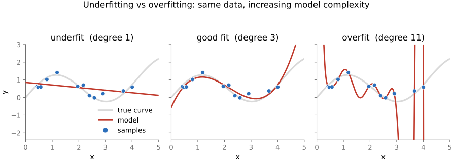
Overfitting and the bias–variance trade-off. Fit your model too closely to the measurements and you fit the noise too, so it generalizes badly (Figure 45.2.6⛶ fullscreen: a low-order fit underfits, a sky-high-order polynomial overfits, something in between is right). The dials are model capacity, the regularization strength, and a proper held-out validation set to tell which side you're on. Note that $\lambda$ here is the same dial as the regularization $\lambda$ above, and this is precisely the bridge to machine learning, where overfitting is the central worry.

💡 Big lesson. Because the measurement genuinely loses information, the prior is not optional: it is what makes recovery possible at all. This is the sense in which, across the book, "quantization is rarely the issue; the prior is" (Big Lessons): what limits a reconstruction is usually not the bits you kept but the assumptions you bring. The standing references here are Boyd & Vandenberghe's Convex Optimization, chapter 7 of Deisenroth, Faisal & Ong, and Strang on least squares and gradient descent. This whole machinery gets a chapter of its own in Single-image computational photography.

45.2.4 Probability and information theory🔗⧉

Noise is random, so measuring it and removing it is probability. The best estimate given a noisy measurement and a prior is Bayes, and it leads to the same optimization problem as the previous section. And how many bits an image fundamentally needs is information theory, which is the theory behind compression. Keep it light here; the goal is fluency, not rigor.

Random variables, distributions, expectation, variance. A pixel reading is a random variable scattered around the true value. For an unbiased calibrated measurement, its mean $\mu = E[X]$ is the underlying signal; its variance $\sigma^2 = E[(X-\mu)^2]$ (and its square root, the standard deviation $\sigma$) is the noise. Two facts do most of the work downstream: expectation is linear ($E[aX+bY] = aE[X]+bE[Y]$ always), and the variances of independent quantities add.

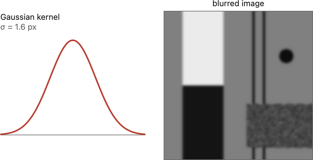
The two distributions we actually use. The Gaussian $\mathcal N(\mu,\sigma^2)$, the bell curve (Figure 45.2.7⛶ fullscreen), with its $\pm\sigma$ width, is everywhere: it models read noise, it is what the central limit theorem pushes sums toward, and it is the reason squared error is the "natural" loss (Gaussian noise $\Leftrightarrow$ least squares). The Poisson distribution governs photon counting: light arrives as discrete photons, and a count with expected value $N$ has variance $N$ and standard deviation $\sqrt N$ under the Poisson model. The consequence is a central fact about sensor noise: signal-to-noise ratio is worse in the shadows, where few photons land (Chapter 2.2, Image formation and linear perspective).

Independence and averaging. Average $N$ independent, equally noisy measurements of the same thing and the variance drops by a factor of $N$, so the std drops by $\sqrt N$. This one fact is the engine of an enormous amount of computational photography: it is why we stack frames, why a longer exposure or a bigger pixel is cleaner, and the seed of the whole "quality through quantity" thread.

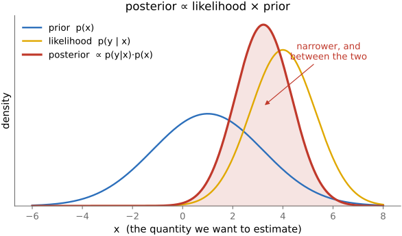
Conditional probability and Bayes. Bayes' rule, $p(x\mid y) \propto p(y\mid x)\,p(x)$, says the posterior (what we believe about the scene $x$ after seeing measurement $y$) is the likelihood (how the measurement is produced, the noise model) times the prior (what scenes are plausible), suitably normalized (Figure 45.2.8⛶ fullscreen). Taking the most probable $x$ (MAP estimation) and writing it in $\log$ form turns it into $\min_x [-\log p(y\mid x) - \log p(x)]$, which is exactly the "data term + prior" loss of the optimization section. The two viewpoints are one thing seen twice. Discounting the illuminant (white balance), denoising, and demosaicking are all, at heart, Bayesian estimates.

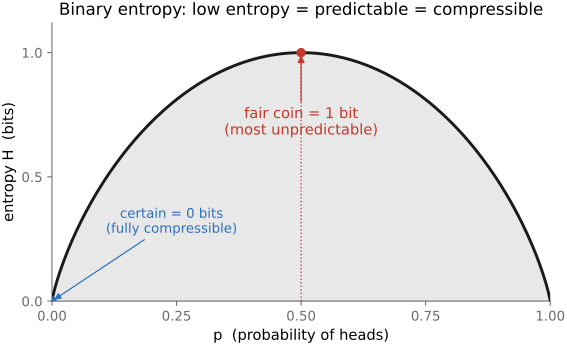
Information and entropy. The entropy $H=-\sum_i p_i\log_2 p_i$ measures average surprise in bits. It is a lower bound on average lossless code length, approached by efficient coding of long sequences under the source model. It is largest when outcomes are most uncertain: for a single coin flip, $H(p)$ peaks at $p = 0.5$ and vanishes at $p=0$ or $1$ (Figure 45.2.9⛶ fullscreen). Low entropy means predictable means compressible: that is the theory beneath the entropy coding in Chapter 8.11, File formats and compression. (Mutual information, "bits shared between two variables," is the same idea applied to dependence.) Kept light, this is enough to see why JPEG can shrink a photo of the sky and why why unpredictable noise is difficult to compress losslessly; lossy JPEG can still shrink it by discarding information: structure is low-entropy, noise is high-entropy.

💡 Big lesson. Averaging $N$ independent samples cuts the noise std by $\sqrt N$: quality through quantity, the seed of all multi-shot imaging (Part 13, Denoising, Big Lessons). For the deeper story, MacKay's Information Theory, Inference, and Learning Algorithms (free, and superb on exactly the Bayes-meets-coding view above) and chapter 6 of Deisenroth, Faisal & Ong are the companions.

45.2.5 Machine learning and deep learning🔗⧉

Learned methods now dominate denoising, demosaicking, super-resolution, tone mapping, and much else, so a reader needs the vocabulary. It is the same vocabulary as the optimization section, scaled up. Supervised learning is fitting a function by minimizing a loss; neural networks are composable differentiable building blocks; and training is gradient descent driven by backprop. What changes is the prior: instead of hand-designing it, we learn it from data.

Supervised learning = curve fitting, scaled up. Given example pairs $(x_i, y_i)$, find a model $\hat y = f_\theta(x)$ whose parameters $\theta$ minimize the average loss

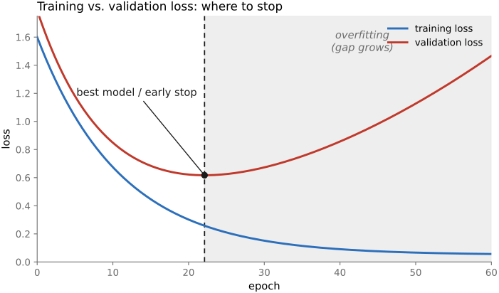
That is precisely the regression of two sections ago, now with millions of parameters instead of a handful. Split the data into train / validation / test; the goal is generalization to new inputs, not memorization of the training set, the overfitting worry of Figure 45.2.6⛶ fullscreen, made central.

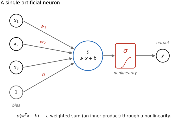
The artificial neuron and layers. A single neuron computes $\sigma(w^\top x + b)$: a weighted sum of its inputs (an inner product, the linear-algebra section again), shifted by a bias $b$, then squashed through a nonlinearity $\sigma$ such as a ReLU or sigmoid (Figure 45.2.10⛶ fullscreen). Stack many neurons into a layer, stack layers into a multilayer perceptron, and a deep network is a long composition $f_\theta = f_L \circ \cdots \circ f_1$ of such blocks. The nonlinearity between layers is what makes the stack more expressive than one big matrix: without it the whole thing would collapse to a single affine map when biases are included.

Training = gradient descent + backprop. We minimize $\mathcal L(\theta)$ by stochastic gradient descent, $\theta \leftarrow \theta - \eta\,\nabla_\theta \mathcal L$. The gradient $\nabla_\theta\mathcal L$ is computed by backpropagation, which is just the chain rule (the calculus section) applied efficiently through the layer-by-layer composition. In practice an autodiff framework like PyTorch does this for you: you write the forward computation, and the gradients come back for free (the programming section, next). The whole training loop is "predict, measure the loss, backprop, step downhill," repeated over minibatches.

Convolutional networks: the imaging-native architecture. The workhorse for images is the convolutional neural network: filters that are local (each output looks at a small neighborhood) and weight-shared (the same filter slides across the image), giving translation equivariance away from boundaries for stride-one convolutions; striding and padding qualify that property. In other words, a CNN learns convolutions (Chapter 6.2, Convolution) instead of having them hand-designed: a natural fit for images. For image-to-image tasks (denoise, demosaic, super-resolve) the dominant shape is an encoder–decoder / U-Net, which processes the image across scales, echoing the pyramids of Chapter 6.6, Pyramids and wavelets. We keep this brief and forward-point to the advanced books for the real depth.

What changes versus classical methods. The skeleton is unchanged: still "loss = data-fit + prior." What changes is that the prior is now learned from a dataset rather than written down by hand. The upside is state-of-the-art quality; the costs are real: appetite for data and compute, brittle failure modes, and (the one to flag for imaging) hallucinated detail, where the model invents plausible texture that was never measured. That last matters ethically and evidentially, not only for quality, and is taken up in Chapter 40.1, Human factors and the art of photography.

💡 Big lesson. A learned method swaps a hand-tuned regularizer for a prior learned from data, the very same "data-fit + prior" loss of the optimization section, now data-driven (Optimization and regression). The companions are Prince's Understanding Deep Learning (free, modern, beautifully illustrated) and Goodfellow, Bengio & Courville's Deep Learning for the deeper standard. This section is the hinge between the book's "hand-designed operator" chapters and its "learned operator" ones across Books 2–3.

45.2.6 Programming: Python, C++, and PyTorch🔗⧉

This book ships in two languages from one source. It renders as either a Python book or a C++ book (Book Generation Process), so this section sets expectations rather than teaching a language. The mental model is short: Python/NumPy for clarity and prototyping, C++ for performance, PyTorch for tensors plus autograd plus GPU. The one idea that unifies all three is the one from the linear-algebra section: an image is an array, and operations can be expressed over arrays, whether implemented as compiled pixel loops or library calls.

Why two languages. Python with NumPy reads almost exactly like the math (array operations, vectorization, broadcasting), which is why it's the language for explaining and prototyping. C++ is the same operations when speed and memory matter: the camera ISP, real-time pipelines, Halide-generated kernels. The dual-language build lets a listing exist once and render in whichever language the reader chose; this section is the shared mental model under both.

Images as arrays / tensors. An image is an $H \times W \times C$ array: a NumPy ndarray, a C++ buffer, or a torch.Tensor. In ordinary Python, prefer array operations implemented by optimized libraries over scalar Python loops: img * 0.5 to darken, a + b to blend, a slice to crop. That is the linear-algebra "image as a vector" view made executable, and it is both clearer and far faster than a Python for-loop. Know your indexing, slicing, and broadcasting rules; and inspect the actual strides: NumPy commonly uses row-major storage, but views, channel layouts, and other frameworks can differ, so loop order and access pattern decide cache behavior: a thread we pick up in Part 29, Making computational photography code fast.

PyTorch in one paragraph. A PyTorch tensor is an array that can live on CPU or GPU, plus automatic differentiation (autograd). With gradient recording enabled, supported operations involving tensors that require gradients build a graph. loss.backward() accumulates gradients into the relevant leaf tensors; it does not automatically differentiate every input or nondifferentiable operation: the backprop of the ML section, automated. This is why modern imaging code is written in PyTorch even when nothing is being learned: you get free derivatives (for any optimization, not just training) and GPU execution for supported operations when tensors are placed on an available device.

Pointers to practice. The dual-language listings, the book's imageops / figstyle conventions (Conventions, Notation & Style), and the warmups in Exercises & Experiments make all of this concrete. Start with the simplest possible loop: load an image, confirm it's just a NumPy array of numbers, do some arithmetic on it, and save it back out. Everything else in the book is that, scaled up.