45.4 Problem Set 1 — Image class, point operations, and color🔗⧉

Problem Set 1: Basic Image Processing. Due Wednesday September 23, 9:00pm.

45.4.1 Summary🔗⧉

• The Image Class
• Brightness and Contrast
• More Image Class Methods
• Colorspaces
• Spanish Castle Illusion
• White Balance

45.4.2 The Image Class🔗⧉

Throughout this course we will be using the Image class introduced at the end of the last pset. The Image class specification is given in Image.h. Images are three dimensional arrays (width $\times$ height $\times$ color channel) that store pixels as a vector of floats called image_data. In memory, the pixels in the image are stored sequentially in row-major order in three adjacent color planes. That is, the distance (or stride) between adjacent values in the same row in image_data is equal to 1. The stride between adjacent values in the same column is equal to the width of the image and the stride between the different color channels at the same pixel is width$\times$height. You can use the method int stride(int dimension) to compute these values.

image_data is a C++ vector, which is essentially an array which manages its own memory (as seen in pset0). You can access elements of it using brackets. For instance, image_data[0] returns the front element in the vector. More information about vectors can be found at <http://www.cplusplus.com/reference/vector/vector/>.

For images that correspond to pictures, the floating points in image_data will be between $0$ and $1$. There is nothing guaranteeing that the values of image_data stay in this range and there may be times when you want to use the Image class to store intermediate data that doesn't correspond to pictures, in which case the range is not meaningful. When the image is written to a file, it will assume the data lies in this range and will clip values outside of the range to one of the endpoints.

You can use the Image write method to write images to .png files. For example:

my_im.write("./my_image.png");

Then, you can view them in your favorite image viewer. This may be useful for debugging. Alternatively, if you don't feel like providing a filename, you can use my_im.debug_write() to write an image to an automatically named file. This might make debugging easier.

Pixel Accessors and Setters🔗⧉

You are going to implement the accessor and setter operators for pixel values in the image. We adopt the convention that the elements are accessed via the () operator. This is contrary to C++ convention, but will allow us to match the syntax of Halide (<http://halide-lang.org/>), which we will use at the end of the semester to write fast image processing code. That is, the pixel at location $(x,y)$ in the third color channel of my_im is accessed via

my_im(x,y,2);

Note that there are three channels, but they are index using 0-based-index, that is the channels are accessed as $[0,1,2]$.

Implement three accessors with $0$-indexing and bounds checking to make sure the input is valid. If the input is not valid, throw an exception using the command throw OutOfBoundsException();.

In Image.cpp implement:

• 1.a number_of_elements() : returns the number of elements in the image. An RGB (3 color channels) image of $100 \times 100$ pixels has $30000$ elements.
• 1.b my_im(x) : returns the value of image_data at location $x$ as long as $x$ is less than ($<$) the total number of elements and at least ($>=$) 0. You need to implement the functions const float & operator()(int x) const float & operator()(int x) with identical code. Use number_of_elements() for bounds checking.
• 1.c my_im(x,y,z) : returns the value at location $(x,y)$ in the $z$-th color channel. You need to implement the functions const float & operator()(int x, int y, int z) const float & operator()(int x, int y, int z) with identical code. Use width(), height() and channels() for bounds checking.
• 1.d my_im(x,y) : returns the value at location $(x,y)$ in the $0$-th color channel. You need to implement the functions const float & operator()(int x, int y) const float & operator()(int x, int y)

Creating Basic Images/Shapes🔗⧉

It will be useful for testing and debugging to have basic images and shapes in our image class. Currently when the Image class constructor is called it generates an all zeros image (when no filename is specified).

In Image.cpp implement:

• 2.a set_color(float r, float g, float b) : which sets all the pixels of the image to the specified values. That is, all pixels in the first channel should get the value r, pixels in the second channel should get values g, etc. Note that pixels should only be assigned if the channels are valid. I.e., if the number of channels is equal to 1, ignore the g and b values.
• 2.b create_rectangle(int xstart, int ystart, int xend, int yend, float r, float g, float b) : which sets the pixels inside the rectangle [xstart, ystart] $\rightarrow$ [xend, ystart] $\rightarrow$ [xend, yend] $\rightarrow$ [xstart, yend] (inclusive) to the specified color. If the rectangle coordinates are not valid, throw an out of bound exception (throw OutOfBoundsException()). As above, only set the color of valid image channels.

Note that both of these functions have default arguments <http://en.cppreference.com/w/cpp/language/default_arguments> (see their declarations), so that you can call them with a subset of the channels if appropriate.

And now for a treat, in a1.cpp implement:

• 2.c Image create_special() which returns an image where the following operations have been performed:

• Create an image of size 290 $\times$ 150 $\times$ 3.
• Set all pixels to white (1.0, 1.0, 1.0)
• Draw rectangles: with coordinates (zero-based index) and colors:

$$ \begin{array}{ccc} Start (x,y) & End (x,y) & Color (r,g,b) \\ \hline (0, 0) & (31, 149) & (0.64, 0.12, 0.20) \\ (52, 0) & (83, 102) & (0.64, 0.12, 0.20) \\ (103, 0) & (134, 149) & (0.64, 0.12, 0.20) \\ (155, 0) & (186, 30) & (0.64, 0.12, 0.20) \\ (155,48) & (186, 149) & (0.55, 0.55, 0.55) \\ (207, 0) & (289, 30) & (0.64, 0.12, 0.20) \\ (207,48) & (238, 149) & (0.64, 0.12, 0.20)\end{array} $$

• 2.d Run the function Image create_special() and save the output image. What does the function create? (Answer in the submission form).

6.8370 Only:

In Image.cpp implement:

• 2.e create_line(int xstart, int ystart, int xend, int yend, float r, float g, float b) : which sets the pixels of the line segment [xstart, ystart] $\rightarrow$ [xend, yend] to the specified color. There are more than one way to draw a line. We will accept the solution as long as it is not too far off. Your solution will have to support lines in arbitrary direction. Start/end points are inclusive bounds.

45.4.3 Brightness and Contrast🔗⧉

Now for the fun part. Once we have these accessors, we can perform simple operations like increasing the brightness or contrast of an image.

• 3.a Implement the function brightness in a1.cpp, which multiplies the pixels in an image by the value factor. Make sure to create a new image and return that rather than modifying the input image. This is good practice in case you want to use the input again.
• 3.b Implement the function contrast, which increases the contrast of an image around a specified midpoint by the value factor. That is, you should apply the following function to every pixel's value

$$ I_{out} = {\tt factor} \times (I_{in} - {\tt midpoint}) + {\tt midpoint}. $$

You can test your functions on the included Input/Boston_underexposed.png and Input/Boston_low_contrast.png. The input images have low brightness or low contrast - you can use your brightness or contrast function to increase the brightness and the contrast.

45.4.4 More Image Class Methods🔗⧉

We have added operators for the Image class that allow you to add, subtract, multiply and divide images element-wise in the same way as built-in types like float. That is, you can now do things like

Image im1(640,480,3), im2(640,480,3);
float a = 2.0, b = -1.0, c = 0.0;
Image out1 = im1 + im2;
Image out2 = im1 - b;
Image out3 = a * im2;
Image out3 = im1/c; // This will throw a DivideByZeroException();

You can inspect the code in Image.cpp. When an operator is used with two images, they must be of the same size or a MismatchedDimensionsException() will be thrown.

We also added an InvalidArgument exception that you can throw using throw InvalidArgument(); if you want to handle arguments that you think are not valid. Since this isn't a software engineering class, we won't test you on whether you handled invalid input correctly. If you do choose to use this exception, make sure the input is actually invalid. The optional InvalidArgument handling discussed here is separate from the bounds checks explicitly required above.

45.4.5 Colorspaces🔗⧉

In this section, you will implement several functions related to changing an image from RGB colorspace to other colorspaces.

• 4 Implement the function color2gray in a1.cpp, which performs a weighted average across color channels of an input image im and outputs a grayscale image. The weights are in the length 3 vector weights. The returned image should be a two dimensional image with one color channel (instead of three color channels).

Luminance-Chrominance🔗⧉

When we convert a color image to grayscale using the color2gray function, we get the luminance of the image, but lose the color information or chrominance $(kr,kg,kb)$. You can compute this chrominance by dividing the input image by the luminance. Once the luminance and color information have been separated, you can modify them separately to produce interesting effects.

Which values to use. Use the stored RGB values and the supplied coefficients for these exercises. No additional gamma conversion is required unless explicitly requested. For encoded RGB, the weighted grayscale value is a luma-like quantity rather than physical luminance.

• 5.a Implement the function lumiChromi in a1.cpp. This function should return a vector of two images, a luminance image and a chrominance image. The luminance image should be the first element in the vector and it can be computed using color2gray with the default weights.
• 5.b Implement the function brightnessContrastLumi in a1.cpp, in which brightness and contrast of only the luminance of the image should be modified. Decompose the image into luminance and chrominance and then modify the luminance. Apply brightness first, then contrast to the resulting luminance. Recombine the modified luminance with the chrominance by multiplying to produce the output image.

We can think of the luminance as the “light intensity”, and the chrominance as the “color information”. Therefore, if the luminance of a specific pixel is 0, then a good assumption is that the pixel has no color (as far as images are concerned).

YUV🔗⧉

Another representation of an image that separates overall brightness and color is the YUV colorspace. An RGB image can be converted to and from a YUV image using the matrix multiplications

• 6.a Implement the functions rgb2yuv and yuv2rgb, which convert images from one colorspace to the other.
• 6.b Implement the function saturate(const Image & im, float factor), which multiplies the U and V channels of an image by a multiplicative factor. The input and returned image should be in RGB colorspace.

In YUV space, the elements of the image won't necessarily be in the range $0$ to $1$. If you try to write the image, the image write function will assume the input is an RGB image and it will round values outside of the range to the endpoints. Keep this in mind when testing and debugging your functions. Up to rounding errors, the functions rgb2yuv and yuv2rgb will be inverses of each other.

Discussion🔗⧉

The chrominance-luminance and the YUV conversions perform similar operations: they decouple an image's “intensity” from its “color.” There are, however, important differences. YUV is obtained by a purely linear transformation, whereas our chrominance-luminance decomposition requires a division. Furthermore, the latter is overcomplete (we now need 4 numbers), while YUV only requires 3. YUV does a better job of organizing color along “opponents” and the notion of a negative is more perceptually meaningful. On the other hand, the separation between “intensity” and “color” is not as good as with the ratio computation used for luminance-chrominance. As a result, modifying Y without updating U and V changes not only the luminance but also the apparent saturation of the color. In contrast, because the luminance-chrominance decomposition relies on ratios, it preserves colors better when luminance is modified. This is because the human visual system tends be sensitive to ratios of color channels, and it discounts constant multiplicative factors. The “color” elicited by $r$, $g$, $b$, is the same as the color impression due to $kr$, $kg$, $kb$, only the brightness/luminance is changed. This makes sense because we want objects to appear to have the same color regardless of the amount of light that falls upon them.

Gamma-Encoding🔗⧉

A camera sensor measures light, and the camera then turns that measurement into a stored image with a limited number of levels per channel, typically 256 (8 bits). Those are two different things: the sensor data, and the encoded image written to a file. Pixel values are normalized to $[0,1]$. The supplied photographs are gamma encoded except where stated otherwise.

Quantization maps a continuous range of values to a few levels. With two bits, we can represent four different values. First assign each input value to one of four equal-width bins, numbered 0 through 3. Then represent that bin by the corresponding float value 0, $1/3$, $2/3$, or 1:

The input value 1 belongs to the last bin; it must not create a fifth bin. The bins are $1/4$ wide while the returned values are $1/3$ apart, and those are different quantities. We still store floats in this exercise, so we reduce the number of possible values without reducing memory usage.

Uniform (also known as linear) quantization spreads its levels evenly over the range. However, humans perceive light in a non-linear manner (where mostly multiplicative effects or ratios of intensities matter). As a result, images are usually gamma encoded before they are quantized. Gamma encoding maps linear intensity $x$ to $y = x^{1/\gamma}$; we then quantize $y$. Here $\gamma$ represents a power controlling the transformation (typically a value around $2$). This encoding spends more levels on the part of the range that humans are more sensitive to and fewer where it matters less.

Most images we interact with are already in this gamma space. However, some image processing steps (i.e. deblurring, HDR merging) work better when the data is in linear space, so the image first needs to be decoded before being processed. When displaying, the image needs to be re-encoded into gamma space, as most devices assume that the data is gamma encoded and linear images might appear a bit dark and low contrast.

• 7.a Implement the function Image gamma_code(const Image &im, float gamma) in a1.cpp which adjusts the values of the input image by the specified gamma. Hint: a good self-check here is to write the output of this function when given our raw image (./Input/skies_and_trees.png, which is stored in linear light and so looks dark and flat until you encode it) as input and a reasonable guess for gamma. Did the colors improve?
• 7.b Implement the function Image quantize(const Image &im, int bit) in a1.cpp which uniformly quantizes the pixel values (in the range [0,1]) to bit bits (the output should also be in the range [0,1]). Hint: consider scaling up the input values by the necessary amount, extracting an integer bin number and scaling back to [0,1]. Use the convention from the two-bit example above: with $n = 2^{\mathtt{bits}}$ levels, the integer bin is $\lfloor n x \rfloor$, except that $x = 1$ goes into the last bin $n-1$, and the returned value is the bin number divided by $n-1$. So 0 maps to 0 and 1 maps to 1. (Other conventions, such as returning the center of each bin, are reasonable elsewhere; this exercise uses this one.) Note: this is fake' quantization as we have not saved any space (still using the same number of floats`) in the range [0,1]; however, the number of unique values should be reduced to $\leq 2^\mathtt{bits}$.
• 7.c Put it all together, implement vector<Image> gamma_test(const Image &im, int bits, float gamma) in a1.cpp :

• Create im1 by quantizing the input image.
• Create im2 by linearizing the input image, quantizing, then re-encoding the image back into gamma space.
• Return im1 and im2 as a vector

• 7.d Try the function gamma_test on ./Input/night_lanterns.png and then on ./Input/cave_pool.png, both with 6 bits and gamma 2.2. These are ordinary gamma-encoded photographs, which is what gamma_test expects: it does the linearizing itself. Both were chosen because a large part of each frame is smooth and dark, and that is where six bits runs out first. Look at the night sky above the lanterns, and at the shaded rock and the water in the cave. Take a look at generated images. What are the perceptual difference between the images? Which image looks better? (Answer in the submission form).

45.4.6 Spanish Castle Illusion🔗⧉

You can use the colorspace functions you implemented to implement the Spanish castle illusion, which you can read more about at <https://annrichmanart.com/blog/color-theory-part-1-how-do-we-see-color> (see the Previously Viewed Subjects May Impact Color Perception section)

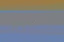
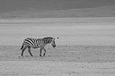
Given an input image, you should create two images. The first image has a constant luminance (Y) and its chrominance are the opposite of the input's chrominance (-U and -V). The second image is a black-and-white version of the original, i.e.\ both U and V should be uniformly zero. In the first image, set the luminance to be $0.5$. To help people focus on the same location, add a black dot in the middle of both images. If image has dimensions $w\times h$, make sure that the black dot is at the $0$-indexed location ${\tt floor}(w/2), {\tt floor}(h/2)$.

• 8 Implement the function spanish, which takes an input image and returns a pair of images that can be used within the Spanish castle illusion. Make sure the gray scale image is the second element in the returned vector.

You can try out your function on the included castle_small.png and zebra.png or your own images.

45.4.7 White Balance🔗⧉

You will implement a function to white balance an image. We will be using the gray world assumption, in which the mean color of a scene is assumed to be gray. Specifically, you want to white balance an input image by multiplying each channel of the image by a factor, so that the average value of each of the three channels of the output image is the same. It may be helpful to write a function that computes the average value of each of the three channels.

• 9 Implement the function grayworld in a1.cpp, which automatically white balances the input image by using the gray world assumption. Make the average value of each of the three channels of the output image equal to the average value of the green channel of the input image.

You can try out your function on the include flower.png image.

6.8370 Only

• 10 For what kind of images do you think white balancing with the gray world assumption will not produce a good result? (Answer in the submission form).

45.4.8 Submission🔗⧉

Turn in your files to the online submission system and make sure all your files are in the asst directory under the root of the zip file. If your code compiles on the submission system, it is organized correctly. The submission system will run code in your main function, but we will not use this code for grading. The submission system should also show you the image your code writes to the ./Output directory

In the submission system, there will be a form in which you should answer the following questions:

• How long did the assignment take? (in minutes)
• Potential issues with your solution and explanation of partial completion (for partial credit)
• Any extra credit you may have implemented and their function signatures if applicable
• Collaboration acknowledgment (you must write your own code)
• What was most unclear/difficult?
• What was most exciting?