36.8 Feed-forward (amortized) 3-D: skip the per-scene optimization⧉
The radiance fields of the previous chapter are photorealistic and slow, and they share a structural weakness with the classic pipeline before them: they start from zero for every scene. NeRF and 3DGS overfit a fresh representation to each new set of photos by a per-scene optimization; the classic pipeline runs its whole feature-matching-and-bundle-adjustment chain anew each time. The newest line of work asks a different question: can we pay the cost once?
36.8.1 Amortization: pay once, reuse forever⧉
The idea is amortization, borrowed from machine learning's broader playbook. Instead of solving an optimization problem per instance, train a network across many instances so that, at test time, solving a new instance is a single forward pass. Applied here: train a network on enormous quantities of scenes (with known 3-D), and then reconstruction of a new scene becomes one forward pass, taking seconds rather than minutes or hours (Figure 36.8.1). "Pose structure-from-motion as a supervised learning problem," in a phrase. The slow optimization does not disappear; it is moved offline into training, paid once, and amortized over every future scene the model sees.
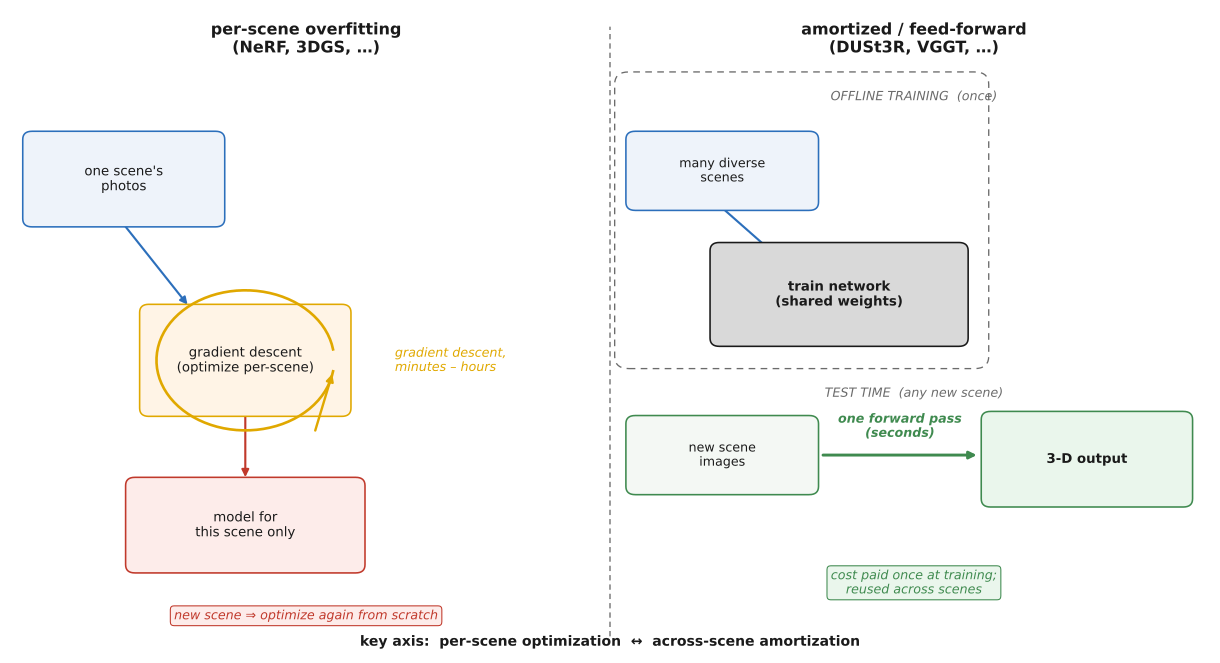
A second advantage is that the method is structurally simpler. The classic pipeline is a long chain of hand-built stages, each a separate algorithm with its own failure modes and its own parameters, and errors propagate down it. An amortized network can replace much of that chain with direct prediction. Practical systems may still extract correspondences, estimate poses, align pairwise outputs globally, or run bundle adjustment. The network predicts 3-D directly.
36.8.2 The line: DUSt3R, MASt3R, VGGT⧉
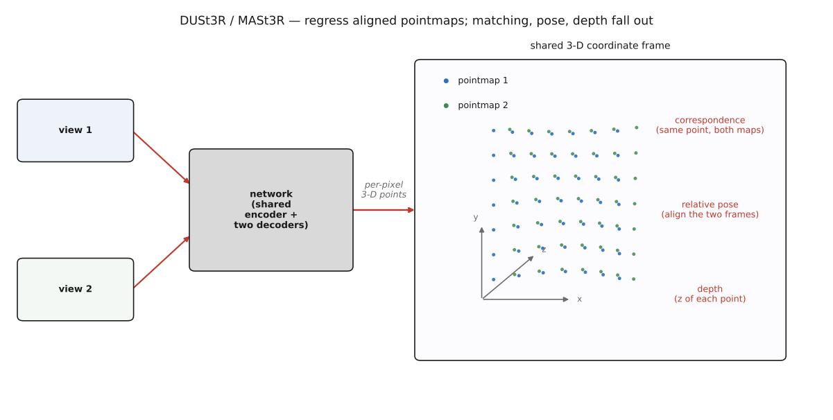
DUSt3R Wang et al. 2024 (DUSt3R) is the clearest statement of the idea. Feed it two images and it directly regresses, for each image, a per-pixel point map (a 3-D point for every pixel) with both point maps expressed in one shared coordinate frame. That last clause is the trick: because the two point clouds already live in the same frame, correspondence, relative pose, and depth all read straight off the aligned points (Figure 12.6.3). Two pixels that map to the same 3-D point are a correspondence; aligning the two frames gives the relative camera pose; a point's $z$ is axial depth only after expressing it in the relevant camera's frame. DUSt3R's second-view point map is expressed in the first camera's frame, so its stored $z$ is not directly second-camera depth. There is no explicit feature detection, no matching stage, no calibration assumed; the network learned to do all of it implicitly. Camera parameters can be estimated from these correspondences between image coordinates and predicted 3-D points. With many input pairs, DUSt3R also uses global alignment to reconcile their coordinate frames and scales.
MASt3R Leroy et al. 2024 (MASt3R) adds a dense 3-D matching head on top of DUSt3R for higher precision and sub-quadratic matching at scale, and downstream systems use these predictions for SLAM. Such systems also need tracking, mapping, and consistency machinery beyond one pairwise forward pass. VGGT Wang et al. 2025 (VGGT) generalizes from pairs to many views in a single feed-forward transformer: built on DINO image features with alternating frame-local and global attention, it emits camera parameters, depth maps, point maps, and 2-D point tracks all at once, for a whole set of images, in one pass, the entire SfM output as a single network prediction. (Follow-ons such as pi³ remove VGGT's privileged-first-frame bias, making scene prediction permutation-equivariant: permuting inputs correspondingly permutes per-view outputs, rather than privileging the first view.)
36.8.3 The observation, and the loop it closes⧉
Here is the observation that ties the part together. A point map is, per image, just a depth map unprojected into 3-D. So a feed-forward reconstructor is a monocular-depth estimator made multi-view-consistent: predict per-pixel 3-D for each image such that the images agree in a shared frame. Even perfect per-image depth does not supply camera intrinsics, relative poses, or cross-view registration for free. The shared-frame prediction is additional work, not merely a relabeling of independent depth maps. That is exactly the loop back to Chapter 36.3, Monocular depth estimation (one image → depth): monocular depth and feed-forward 3-D are closely related tasks, with multi-view consistency and camera estimation adding constraints and outputs.
36.8.4 The trade, and the data dependency⧉
Feed-forward methods trade ultimate precision for speed, generality, and few-view robustness. A careful per-scene NeRF/3DGS optimization, given enough well-posed views, can improve on a feed-forward initialization; but an amortized model is attractive when you have few views, no poses, or a time budget of seconds. The two paradigms are increasingly combined: use a feed-forward model for instant poses and a coarse 3-D, then (optionally) refine with a short per-scene splat optimization. Methods such as InstantSplat do exactly this.
The caveat is the data dependency. These models need supervision, often millions of images with known 3-D, and that ground truth comes from simulation (with exact geometry for the renderer but a real domain gap), depth sensors, or classical SfM/MVS reconstructions (real scenes, but the labels are only as good as COLMAP made them). So the old pipeline does not die; it survives as the teacher that labels the data the new models learn from. The brittle hand-built chain we dissolved into a network is the very thing that trained the network.