34.12 Polarization imaging⧉
Along with intensity and spectrum, light has a polarization state that an ordinary photograph generally does not resolve. It records how much light there is (intensity), and it three-band-samples what color it is (the spectrum, the axis of the previous chapter). But it is completely blind to the third: how the light oscillates, namely the orientation of the electric field as the wave travels, its polarization. That orientation is not a curiosity. It is the difference between glare and the surface beneath it, between the haze in front of a mountain and the mountain, between one tilt of a facet and another. A camera that ignores polarization throws all of that away before you ever think to ask for it.
This is the part's one move again, transplanted to a new axis. We stacked frames along exposure to beat dynamic range, along focus to beat depth of field, along wavelength to recover a spectrum; here we stack along polarization, deferring questions that intensity alone simply cannot answer: is this glare or is it surface?, how far through the haze is that?, which way does this facet face?, to a per-pixel computation long after the shutter has closed (the L13.1 framing, made precise below). And because polarization, like the spectrum, is one of the axes of the full plenoptic signal, the machinery here is the same capture-a-stack-and-combine machinery you have already seen. It is one more demonstration that the part's idea recurs on every axis of light.
Capture the full set, decide later. An ordinary camera collapses the light's oscillation orientation at the instant of capture, exactly as RGB collapses the spectrum, a Chapter 5.8, Photographic representation and its limits that intensity imaging never even tries to lift. Polarization imaging instead records a small stack across polarizer angles and decides afterward what to do with it: the same defer-the-decision move as HDR on the exposure axis, focal stacks on the focus axis, hyperspectral on the wavelength axis, and light fields on the aperture axis, now run along the polarization axis. The cost is the usual one: more captures, a polarizer, and (for the rotating route) a scene that holds still. The gain is that you can ask glare or surface? how far through the haze? which way does it face? per pixel, once the data is already in hand. (Registered as L13.1 in Big Lessons; first appears in this part's introduction; this is its polarization-axis recurrence, and a clean illustration of the plenoptic lesson that the same stack-and-combine machinery recurs on every axis of light.)
34.12.1 What a camera throws away: polarization as a third axis of light⧉
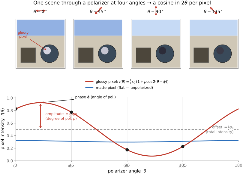
Why is the oscillation orientation worth the trouble of capturing? Because light becomes partially polarized the moment it interacts with the world in certain ways, and that gives the orientation meaning. When light reflects off a dielectric (glass, water, a glossy leaf, skin, a wet road), the polarization depends on incidence angle, refractive index, roughness, and the incoming polarization; it can be strong near Brewster's angle and weak near normal incidence. When it scatters in the atmosphere, the blue sky is polarized in a broad band roughly $90°$ from the sun, a hidden pattern that bees and ants read to navigate, the biological precedent that long predates any camera (Wehner 2001). And the asymmetry that the whole chapter turns on: specular and diffuse reflection can have different degrees and angles of polarization. Multiple scattering often depolarizes body reflection, but diffuse reflection can retain polarization, which is itself used for shape estimation (Figure 34.12.1).
The useful lever is a difference in polarization between components, interpreted under an explicit reflection or scattering model. Where intensity sees one merged value, the polarization stack sees two populations of light that behaved differently, and once you can tell them apart, you can keep one and throw the other away. But none of this is visible in a single ordinary frame. So, exactly as for exposure and wavelength, you capture a stack of it and decide later.
34.12.2 Capturing the stack: rotate a polarizer, or a polarization mosaic⧉
Having decided to fill a polarization stack $I(x,y,\theta)$, the engineering question is the familiar one, and it has the familiar two answers, the same scan-versus-snapshot split of the hyperspectral chapter, trading time against spatial resolution (Figure 34.1.3).
Rotate a linear polarizer: the sequential route. Put a polarizer on the lens, shoot, rotate it, shoot again, classically through $0°, 45°, 90°, 135°$ (three angles suffice to fit the cosine; four is robust). You keep full spatial resolution and may take as many angles as you have patience for, but the capture is sequential in time, so the scene and camera must hold still across the sweep, and hand-held capture needs registration (as in Chapter 13.2, Denoising by averaging). This is the lab-bench, microscope, tripod-on-a-landscape route.
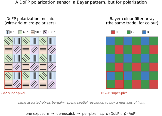
Division-of-focal-plane (DoFP) sensor: the snapshot route. Tile a micro-polarizer mosaic directly over the photosites: $0°/45°/90°/135°$ wire-grid filters arranged in a $2\times2$ super-pixel, a Bayer pattern but for polarization instead of color. One exposure then yields all four angles at once; Sony's IMX250MZR is a production example. The back-illuminated research sensor in (Maruyama et al. 2018) is a separate device. The cost is the obvious one, paid in the same coin as a color CFA: a drop in spatial resolution (and a demosaicking step), because the pixel budget is now split between where and which polarization. This is precisely the assorted-pixels bargain: spend resolution to buy a new axis of light, developed on the sensor side in Chapter 34.1, Assorted pixels.
Either way, from the per-angle intensities you recover, per pixel, the Stokes parameters of linearly polarized light,
where $s_0$ is the total intensity (the ordinary image), and $s_1, s_2$ encode the polarized part. From them follow the two scalar maps the combines below actually operate on: the degree of linear polarization, how polarized the light is on a $0$–$1$ scale,
and the angle of polarization, the orientation of the oscillation,
Equivalently, the per-angle intensity is just Malus's law, $I(\theta) = \tfrac12\,s_0\big(1 + \rho\cos(2(\theta-\phi))\big)$, a cosine in $2\theta$ whose offset is $s_0/2$, amplitude is $s_0\rho/2$, and angular orientation is $\phi$, recoverable by a least-squares sinusoid fit. These linear analyzers do not measure the circular Stokes component $s_3$; full-Stokes capture needs a retarder or equivalent optics. Low $s_0$ makes $\rho$ unstable, and $\phi$ is undefined when the linearly polarized component vanishes. Mosaic samples also need spatial registration/interpolation and analyzer calibration.
34.12.3 Combining images at different polarizations⧉
This is the merge step, the polarization analog of stitching an exposure bracket into a radiance map (the template of HDR merging). When the components have sufficiently different, modeled polarization states, the right combination of the polarized frames isolates or removes a whole component of the image that intensity had hopelessly mixed together.
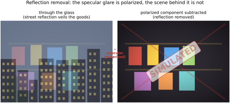
Reflection and glare removal. Shoot through a window, or at a glossy painting, or across a wet street, and the specular reflection comes back strongly polarized while the scene behind it is largely not. Combining the frames to subtract the polarized component makes the window reflection, the glare on the varnish, the sheen on a leaf fade away, revealing the diffuse image underneath (Nayar, Fang & Boult 1997); the earlier polarization-reflectance modeling of Wolff & Boult 1991 set the stage. Near Brewster's angle the surface reflection is almost fully polarized and the suppression is nearly total. This is exactly the photographer's circular-polarizer trick, but done per pixel by computation, recovered from the stack rather than dialled in by hand, and it is the passive cousin of the active reflection separation in Part 35, Computational illumination (Figure 34.12.2).
Specular–diffuse separation. The very same split, used not to remove a layer but to keep both: under the restrictive model of an unpolarized diffuse layer and a fully linearly polarized specular layer, ideal analyzer measurements give $I_\text{diffuse}=2I_\text{min}$ and $I_\text{specular}=I_\text{max}-I_\text{min}$ in pre-analyzer intensity units. Partially polarized specular light leaves an unpolarized remainder that this split cannot distinguish from diffuse light. A clean diffuse layer is useful for many downstream tasks: color constancy, stereo, and recognition all break on specular highlights, and removing them as polarized outliers makes those problems easier.
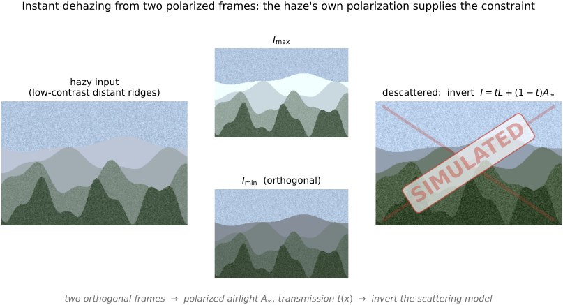
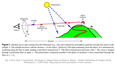
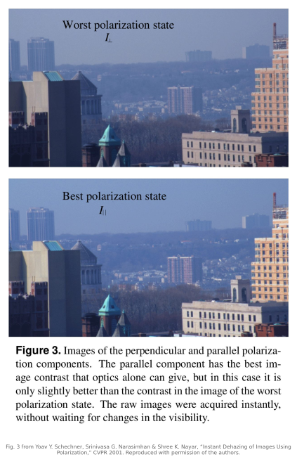
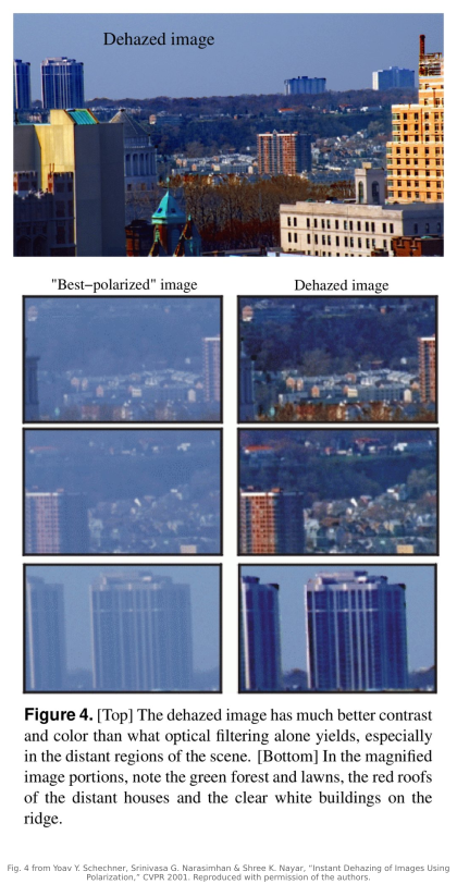
Dehazing and underwater descattering. In haze or water the veiling light (the airlight scattered into the line of sight, or the underwater backscatter) is partially polarized, while the object's own light is much less so. From just two orthogonally-polarized frames, $I_\text{max}$ and $I_\text{min}$, you can estimate the airlight magnitude $A_\infty$ and the per-pixel transmission $t(x)$ from the airlight's degree of polarization, then invert the scattering model
for the clean scene radiance $L$, recovering a descattered, higher-contrast image with transmission providing a depth-related cue under the scattering model (Schechner, Narasimhan & Nayar 2001), the same analysis carried underwater by Schechner & Karpel 2005. It is "instant dehazing" from two frames, requiring assumptions about airlight polarization, illumination, and object polarization; the polarization of the haze itself supplies the missing constraint (Figure 34.12.3).
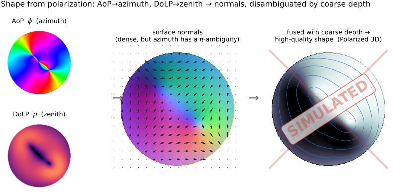
Shape from polarization. The polarization stack is a shape cue. The AoP $\phi$ is tied to a surface's azimuth and the DoLP $\rho$ to its zenith angle, so per-pixel polarization yields a dense field of surface normals, passively, with no light projector and no second viewpoint (Atkinson & Hancock 2006). Alone it is ambiguous: the linear polarization angle is ambiguous modulo $\pi$, and whether you are in the diffuse or specular regime changes the relation. The strong modern result resolves this by fusing the polarization normals with a coarse depth map (from time-of-flight or stereo) so the cheap, low-resolution depth disambiguates the high-resolution-but-ambiguous polarization cue and is upgraded into high-quality normals: Polarized 3D (Kadambi et al. 2015) (Figure 34.12.7).
Every one of these is L13.1 once more: capture the polarization set, then ask the question (glare or surface? how far through the haze? which way does this facet face?) per pixel, long after the light was captured. Polarization takes its place beside exposure (HDR), wavelength (hyperspectral), and aperture (light fields) as one more axis of the plenoptic signal along which you can refuse to decide at the shutter, and defer the decision into software.
Recap: big lessons of this chapter
Capture the full set, decide later. An ordinary camera collapses the light's oscillation orientation at the instant of capture, exactly as RGB collapses the spectrum, a Chapter 5.8, Photographic representation and its limits that intensity imaging never even tries to lift. Polarization imaging instead records a small stack across polarizer angles and decides afterward what to do with it: the same defer-the-decision move as HDR on the exposure axis, focal stacks on the focus axis, hyperspectral on the wavelength axis, and light fields on the aperture axis, now run along the polarization axis. The cost is the usual one: more captures, a polarizer, and (for the rotating route) a scene that holds still. The gain is that you can ask glare or surface? how far through the haze? which way does it face? per pixel, once the data is already in hand. (Registered as L13.1 in Big Lessons; first appears in this part's introduction; this is its polarization-axis recurrence, and a clean illustration of the plenoptic lesson that the same stack-and-combine machinery recurs on every axis of light.)