12.7 Fast matching⧉
Descriptor matching can dominate a large correspondence problem, but feature extraction and index construction also cost time. For a few thousand descriptors, optimized exact search may be competitive. Approximate search trades retrieval quality for speed; evaluate the complete pipeline.
At scale, good-enough-and-fast beats optimal-and-slow; and propagation beats independent search. Two morals braided together. The first is a concession: in high dimensions the exact nearest neighbor costs as much as brute force, so every practical matcher trades a little recall for orders of magnitude of speed, and the operating point on that trade-off is a tuning knob, not a fixed property of the algorithm. The second is an opportunity: when the thing you are matching is spatially coherent (neighboring pixels move together, neighboring patches match to neighboring patches) you should not search for each match from scratch. Let a good answer flood outward to its neighbors, who almost certainly share it. The deepest version of the lesson is the unification at the end: the high-dimensional nearest-neighbor engine that finds correspondences is the engine that runs the bilateral filter and NL-means: matching and filtering are the same search, and an accelerator for one is an accelerator for the other.
12.7.1 Approximate nearest neighbors for sparse descriptors⧉
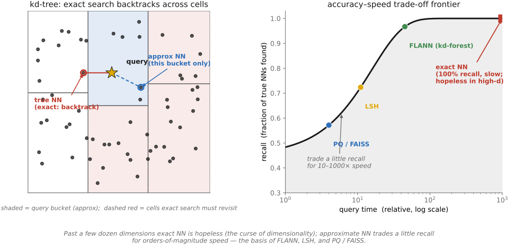
Start with the sparse case: you have two sets of descriptors, say a few thousand SIFT Lowe 2004 vectors per image or a database of a billion, and for each query vector you want the closest one in Euclidean (or Hamming) distance. The textbook data structure is the kd-tree, which recursively splits the point set on alternating coordinate axes and, at query time, descends to the leaf containing the query and then backtracks into neighboring cells that might hold something closer. In low dimensions this backtracking is bounded and the search is logarithmic. In high dimensions it is a catastrophe: the query's true nearest neighbor can sit just across almost any of the splitting planes, so the tree must backtrack through exponentially many cells. By the time you reach the 128 dimensions of SIFT, the kd-tree has quietly become a slow brute-force scan (Figure 12.7.1). This is the curse of dimensionality, and it is the wall every method here is built to get around, not by searching faster, but by searching less, and accepting an approximate nearest neighbor in exchange.
Three families do the work. The first is randomized kd-trees, productized as FLANN (Muja & Lowe 2009, "Fast Library for Approximate Nearest Neighbors", and note whose name is on it: Lowe, the author of SIFT, building the search his own descriptors needed). The trick is to build several kd-trees, each choosing its split dimension randomly from several high-variance coordinate dimensions, and at query time search all of them but only to a bounded number of leaves: you stop early, before backtracking explodes, and take the best candidate found across the trees. You give up the guarantee of finding the true nearest neighbor; you gain a search that stays fast in high dimensions, with recall you dial in by how many leaves you allow. The second is locality-sensitive hashing (LSH) Indyk & Motwani 1998 (LSH): design a hash function with the property that nearby points are likely to collide into the same bucket, then, to answer a query, hash it and scan only the handful of points in its bucket. Where a hash table normally scatters similar keys, LSH deliberately clusters them, so a query only has to scan one small bucket. The third, and the one that scales to billions, is product quantization (PQ) (Jégou, Douze & Schmid 2011): split each vector into chunks, quantize each chunk against its own small codebook, and store every vector as a short tuple of codebook indices. A billion 128-dimensional floats will not fit in memory; a billion 16-byte PQ codes will. Because distances decompose chunk-by-chunk, comparing a query against a code becomes a few table look-ups instead of a 128-term dot product. This is the lineage behind modern vector-search systems such as FAISS Johnson, Douze & Jégou 2021 (FAISS) and ScaNN Guo et al. 2020 (ScaNN).
The point of all three is the trade-off itself, not any single setting. Each knob trades recall (did you find the true nearest neighbor?) against speed and memory, and the right operating point is an application decision, not an algorithm one. A one-off structure-from-motion reconstruction run overnight can afford near-exact search; a phone retrieving an image against a million-item index, in the time it takes to lift it, cannot, and will happily accept ninety-percent recall for a hundred-fold speed-up. When a system today says it does "vector search," this is what it is doing.
12.7.2 PatchMatch: randomized dense correspondence by propagation⧉
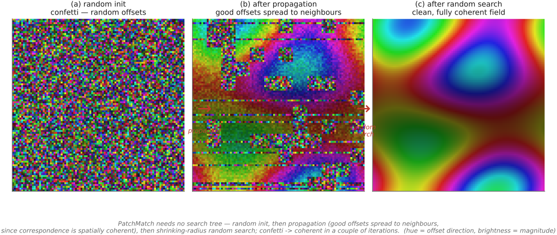
The approximate-nearest-neighbor toolbox above treats every query independently: each descriptor goes off and searches the tree alone. For dense correspondence that independence is wasteful, and PatchMatch (Barnes et al. 2009) is the algorithm that throws it away. The setting is a nearest-neighbor field (NNF): for every pixel in an image, an offset pointing to the most similar patch elsewhere (in the same image, for inpainting and retargeting, or in a second image, for correspondence). Computed naively, that is one tree search per pixel: millions of them. PatchMatch computes it with no tree at all, and converges quickly, by exploiting a single observation: the answer is spatially coherent. Neighboring pixels almost always have similar offsets, because real images are made of coherent regions that move and repeat as wholes. So a neighbor's match is, with high probability, your match shifted by one pixel.
The algorithm is three steps, and the middle one is the whole idea. Random initialization: give every pixel a random offset. This sounds hopeless, but in an image of a million pixels, by sheer luck some of those random offsets are accidentally excellent: a scattering of correct matches hidden in the confetti. Propagation: sweep across the image, and at each pixel test the offsets its already-visited neighbors are using; if a neighbor's offset (applied here) beats the current one, adopt it. A single correct offset can propagate to neighboring pixels in one pass. Alternating the sweep direction each iteration lets good matches propagate up-and-left as well as down-and-right. Random search: to escape local optima, test a few random offsets in a window around the current best, with the window radius shrinking geometrically, using large jumps first to find a better basin and then smaller jumps to refine it. Several sweeps can greatly improve the initial field, but the required count and match quality depend on the images and search objective, fast enough for interactive image inpainting, retargeting, and morphing, the applications taken up in depth in Chapter 21.2, Patch match.
The lesson generalizes well past patches. Propagation beats independent search whenever the answer is spatially coherent, which is why coarse-to-fine pyramids work (a coarse estimate propagates down in scale) and why optical-flow solvers spread motion across smooth regions. PatchMatch is the purest statement of the principle: seed a few good matches and let coherence propagate them (Figure 12.7.2).
initialize one valid target offset for each source patch
repeat for a chosen number of sweeps:
    visit pixels in alternating forward and reverse scan order
    test offsets propagated from already visited neighbors
    retain a candidate only if its target patch is valid and its cost improves
    test random candidates around the best target with shrinking radii
return offsets and matching costs
Specify patch borders and any exclusion region, especially for self-matching. Repetitive textures and independent object motions weaken the coherence assumption; a low patch cost does not establish scene-point identity.
12.7.3 Fast high-dimensional matching by random projection⧉
Random projections and approximate neighborhood search can reduce high-dimensional retrieval cost, but they do not generally preserve every nearest neighbor. Gaussian kd-trees Adams et al. 2009 (Gaussian KD-trees) and the permutohedral lattice Adams, Baek & Davis 2010 (permutohedral lattice) target high-dimensional Gaussian filtering, which aggregates weighted contributions rather than returning a nearest-neighbor identity. The lattice is a structured simplex construction, not a generic random-projection nearest-neighbor index. Chapter 10.1, Bilateral filtering covers that filtering use.
Use a retrieval method when the output is a candidate match or shortlist. Use a Gaussian-filtering method when the output is a weighted aggregate. Similar feature coordinates do not make those objectives interchangeable.
There is still a useful connection to denoising. Bilateral filtering represents samples with spatial and color coordinates; non-local means represents them through patch appearance. Both make similarity a geometric question in a feature space, just as descriptor matching does. The difference is the requested output: one best candidate versus an aggregate of contributions. A data structure can exploit nearby features for either task, but an approximation accurate enough for a weighted sum need not preserve the identity of the nearest sample. This is why the same geometric idea leads to related, rather than interchangeable, accelerators.
Recap: big lessons of this chapter
At scale, good-enough-and-fast beats optimal-and-slow; and propagation beats independent search. Two morals braided together. The first is a concession: in high dimensions the exact nearest neighbor costs as much as brute force, so every practical matcher trades a little recall for orders of magnitude of speed, and the operating point on that trade-off is a tuning knob, not a fixed property of the algorithm. The second is an opportunity: when the thing you are matching is spatially coherent (neighboring pixels move together, neighboring patches match to neighboring patches) you should not search for each match from scratch. Let a good answer flood outward to its neighbors, who almost certainly share it. The deepest version of the lesson is the unification at the end: the high-dimensional nearest-neighbor engine that finds correspondences is the engine that runs the bilateral filter and NL-means: matching and filtering are the same search, and an accelerator for one is an accelerator for the other.